: Sistem Informasi Penelitian Universitas Kristen Satya Wacana J02043

(1)

Linear Prediction and Long Term Predictor

Analysis and Synthesis

Xiaohua Zhou1_{, Banu Wirawan Yohanes}1,2

1_{Faculty of Engineering and Information Sciences,} University of Wollongong, NSW, Australia

2_{Faculty of Electronics and Computer Engineering,} Universitas Kristen Satya Wacana, Salatiga, Indonesia 2_{banu.yohanes@staff.uksw.edu}

Abstract

Spectral analysis may not provide an accurate description of speech articulation. This article presents an experimental setup of representing speech waveform directly in terms of time-varying parameters. It is related to the transfer function of the vocal tract. Linear Prediction, Long Term Predictor Analysis, and Synthesis filters are designed and implemented, as well as the theory behind introduced. The workflows of the filters are explained by detailed and codes of those filters. Original waveform files are framed with Hamming window and for each frames the filters are applied, and the reconstructed speeches are compared to original waveforms. The results come out that LP and LTP analysis can be used in DSPs due to its periodical characteristic, but some distortion might be coursed, which examined in the experiments.

Keywords: Linear Prediction, Long Term Predictor, Synthesis Filter

Ringkasan

Analisis spektral tidak memberikan deskripsi yang akurat mengenai artikulasi wicara. Artikel ini menyajikan penyusunan eksperimen untuk merepresentasikan gelombang wicara langsung dalam bentuk parameter yang bervariasi terhadap waktu. Hal ini terkait dengan fungsi pindah dari saluran vokal. Linear Prediction, analisis Long Term Predictor, dan filter Synthesis dirancang dan diimplementasikan, termasuk dasar teorinya diperkenalkan. Aliran kerja dari filter dijelaskan detil dan juga kode program dari filter tersebut. Gelombang asli dibingkai menggunakan Hamming window dan filter diterapkan pada setiap frame, dan rekonstuksi wicara dibandingkan dengna gelombang asli. Hasilnya LP dan LTP dapat digunakan dalam DSP karena karakteristik periodik, tetapi beberapa distorsi dapat terjadi, yang diamati dalam percobaan.

Kata kunci:Linear Prediction, Long Term Predictor, Filter Synthesis

(2)

Techné Jurnal Ilmiah Elektroteknika Vol. 16 No. 1 April 2017 Hal 49 - 58

properties of speech wave [2]. Therefore, spectral analysis may not provide an accurate description of speech articulation.

It is better to model the speech wave rather than the spectrum to avoid problems within frequency domain methods. For example, Fourier analysis requires along speech segment to provide adequate spectral resolution. Hence, very dynamic speech events cannot be followed accurately. In addition, since voiced speech has periodic nature, then the spectrum between pitch harmonics provides little information.

Partial solution of the problems has been developed using pitch synchronous analysis-by-synthesis methods [3], however they are tedious tasks. This article presents an experimental setup of representing speech waveform directly in terms of time-varying parameters. It is related to the transfer function of the vocal tract [4]. The method presented here may be used to alter acoustic properties of speech signal without loss quality. Other applications are efficient speech transmission and storage, automatic formant and pitch extraction, and speaker and speech recognition.

2. Speech Analysis Model

Speech produced by forcing air from the lungs up through the vocal tract and out through the mouth. Different speech sounds produced by moving the speech articulators, such as vocal folds, tongue, lips, teeth, velum and jaw, into different positions. Speech production model is illustrated in Fig. 1.

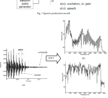
Speech can be classified into two group based on the structure [3]. First category, voiced sounds that have periodic structure and mostly include vowel sounds, e.g. the o in the word coding. Second, unvoiced sounds have mostly random structure and include consonants, such as the p in the word speech. Speech production model uses source filter model, where the source is known as the excitation. Hence, voiced speech has periodic excitation; meanwhile unvoiced speech has aperiodic or random excitation. The period of the signal is the distance between the major pulse peaks and is known as the pitch period, or pitch. The features are illustrated using a narrowband speech signal in Fig. 2(a).

Magnitude spectra derived using short time Fourier transforms (STFT) [3]. The envelope of the speech magnitude spectrum represents the shape of the vocal tract. The envelope of voiced speech shows peaks, as shown in Fig. 2(b). These peaks correspond to the formant frequencies, caused by the resonances occurring in the vocal tract. The unvoiced envelope does not contain such distinct peaks and generally displays a flatter magnitude spectrum, as shown in Fig. 2(c).

(3)

Linear Prediction and Long Term Predictor Analysis and Synthesis Xiaohua Zhou, Banu Wirawan Yohanes

Fig. 1 Speech production model

(a)

(b)

(c)

Fig 2. (a) A narrowband speech signal, (b) Magnitude spectra for voiced section, (c) Magnitude spectra for unvoiced section [6]

2.1. Linear Prediction of Speech

Speech has high correlation between samples and is quasi‐stationary over short durations of up to 30 ms. Both properties are exploited in Linear Prediction (LP) in which LP models the speech signal using a linear filter, the output of which gives a prediction of the current speech sample. The LP model can be described as follows.

(1) where is the prediction of current sample, are previous values, and are

(4)

The speech production model illustrated in Fig 2., time varying digital filter is modeled using linear prediction. Taking z‐transforms of the LP equations and simplifying:

(3) LP coefficients can be derived by minimizing the mean squared prediction error. This error can be calculated using equation as follows.

(4) Here, N is speech segment duration. Generally, N corresponds to between 160 to 200 samples or from 20 ms to 25 ms. It is assumed all samples outside segment are zero, then using a tapered window, for instance Hamming window, to reduce edge effects. This lead to a new formula as follows.

(5) where x(n) = s(n + N) w(n) for 0 ≤ n ≤ N-1 and w(n) is the standard Hamming window.

Minimization of formula (5) involves setting the derivative with respect to each LP coefficient to 0 and solving. For k = i = , , …, p:

Using autocorrelation:

(6) Thus it produces a set of simultaneous equations that are p equations with p unknowns. Then the simultaneous equations can be represented in matrix form as follows.

(5)

where is a p x p autocorrelation matrix values for samples n, is the vector of p LP coefficients, is a vector of p autocorrelation vectors or samples n, and n corresponds to samples within the windowed frame.

A common approach to solving LP matrix is using Levinson-Durbin recursion [7] in O(n2_{) computational time. The recursive process starts with variable}_{E initialization as}

zeroth order autocorrelation. Then for each LPC order from 1 to P calculate ith _k

coefficient, named parcor coefficient, using formula as follows.

for ≤ i ≤ P (8)

This value becomes ith_{LPC coefficient of the i}th_{order LPC vector. For each LPC coefficient}

of them calculate each value using (i - 1)th_{order LPC vector and the i}th_{k value, a}(i)_{(i) = k(i)}

and a(i)_{(j) = a}(i - 1)_{(j) - k(i)a}(i - 1)_{(i - j}) for ≤ _j≤ _{i - 1. Update E using new k value and old value}

E from previous iteration, E(i) = (1 - k(i)2_)E(i-1)_{. At this point, LPC vector of order}_p

obtained by setting each coefficient value to LPC coefficient calculated at pth_{iteration of}

outer loop, a(j) = aP_(j).

2.2. Long Term Prediction

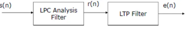
Long Term Prediction (LTP) aims to separate the periodic structure from the random structure of the residual signal obtained following LP of the speech signal. Often, LTP is performed on the residual signal, r(n). Many speech coders include a cascade of an LPC filter and an LTP filter as shown in Fig. 3, with a single excitation source rather than using a switched excitation as input. A simple LTP implementation can be calculated as follows.

(9) where is the predicted residual, M is the pitch, and is the optimum gain term.

The difference between the predicted residual and the original residual is known as the excitation. The excitation can be described by:

Fig. 3 LPC and LTP filters cascade

To find M, search the previous section of residual that most strongly correlates with the current section being analyzed. The optimal gain is found from LTP equation (9). Meanwhile, to find squared LTP prediction error by sum or squares of the difference between the predicted and original residual.

(6)

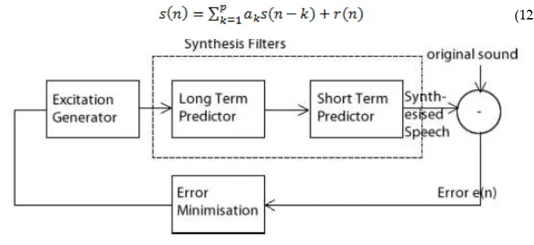
2.3. Synthesis Stage

In this stage, the residual r(n) of original sound is constructed from LTP from λ, M and corresponding previous frame. It is illustrated in Fig. 4. The residual can be calculated using formula as follows.

(11)

After the residual is reconstructed, it can be used to reconstruct the original sound in LP, by following formula.

(12)

Fig. 4 Synthesis stage

3. Result and Analysis

The experiment represented by Fig. 3. The LP and LTP filters work on original speech file sequentially. As the diagram shows, the LP filter takes original speech s(n) as input, and produces the residual r(n), as well as the predictor coefficients A. Then the LTP filter is applied on residual, which produces the excitation, e(n).

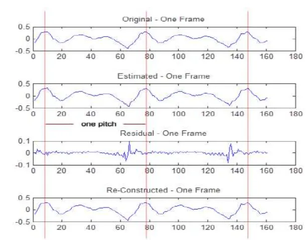
In LP analysis, the optimal coefficients set A is found by Levinson-Durbin recursion algorithm [7], however in this experiment, the Matlab built-in function lpc is used to find the coefficients A. The residual then can be calculated by subtracting estimated signal from original signal.

The result of LP analysis generated by running:

(7)

Fig. 5 Original waveform, estimated waveform, residual, and reconstruction at 67th_frame

The corresponding coefficients A are

The z-transforms of the LP analysis can be written as

And the z-transforms of LP synthesis can be written as

In LTP analysis, for each single frame, the target is to search for the best match frame from previous frames, and then calculate the optimal gain. The previous frame is best match when it minimizes the prediction error E. For each comparison of current frame and M-distance frame in search range, λ is computed by following formula.

(8)

The myLTPcoder function returns the coefficients A, the pitch M, the gain λ, the

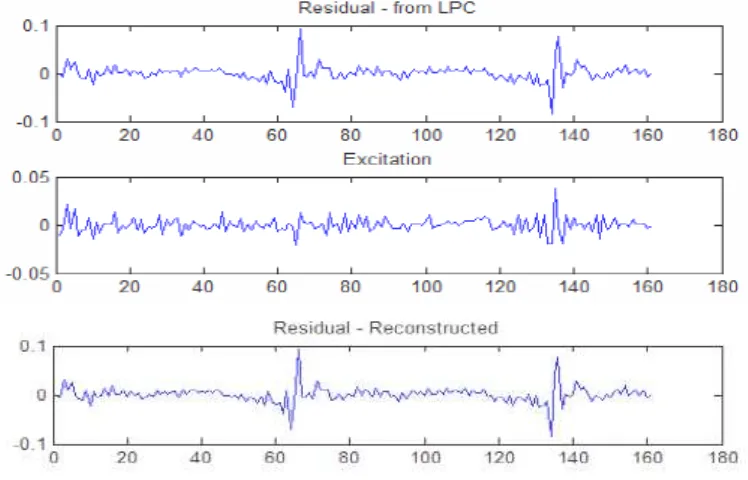
excitation e, the residual and estimated signal from LP analysis. They are parts of LTP analysis. All the outputs will be used in next step when the inverse LTP filter is implemented. The result excitation of the same frame mentioned in Fig. 5 and the reconstructed residual from adding the estimated residual and the excitation e are plotted in Fig. 6.

It can be seen from the figure that the residual can be perfectly reconstructed. There is no obvious difference between original residual signal and reconstructed signal. By examining the excitation e, it becomes very tiny, so it can be easily represented by train pulse sign or other parametric coders in compression.

Fig. 6 Residual from LPC, excitation, and reconstructed residual at 67th_frame

Fig. 7 Excitation at 67th_{frame with sub-frame size is set 50 and search rage is 100}

(9)

The residual is supposed to be reconstructed from the outputs of the LTP analysis. In the experiment, the following code can be used to load the synthesis function:

It reconstructs the original sound by adding the reconstructed residual to estimated signal in LP process. The reconstructed waveform is plotted out.

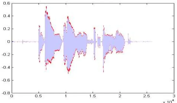
The Fig. 8 shows the difference between reconstructed waveform and the original waveform. It can be seen that there is a slightly difference in amplitude, which is coursed by Hamming windowing process. The signal was multiplied by Hamming coefficients and then they are simple added up with the overlap, the result is not exactly the same as original signal even if no any process applied on windowed signal.

Fig. 8 Difference between reconstructed waveform and the original

4. Conclusion

Several experiments were designed to examine the waveform on time-domain, and also the spectrum on frequency domain. Due to the speech waveform property, the LP can be implemented, which makes the speech compression and transforming much easier. The report analyzed the process of LP analysis and LTP analysis as well as their synthesis filters. The original signal was input to a LP filter which produces the residual and after LTP filter, the excitation become very small values and easy for coding.

(10)

References

[1] L. Flanagan, Speech Analysis Synthesis and Perception, Academic, New York, p. 119, 1965.

[2] E. N. Pinson, Pitch-Synchronous Time-Domain Estimation of Formant Frequencies and Bandwidths, J. Acoust. Soc. Amer. 35, pp. 1264-1273, 1963.

[3] L.B. Rabiner and R.W. Schafer, Digital Processing of Speech Signals, Prentice Hall, New Jersey, 1978.

[4] B. S. Atal, Characterization of Speech Signals by Linear Prediction of the Speech Wave, Proc. IEEE Symp. on Feature Extraction and Selection in Pattern Recognition, Argonne, Ill., pp. 202-209, 1970.

[5] B. S. Atal and M. R. Schroeder, Adaptive predictive coding of speech signals, Bell. Sys. Tech. J., vol. 49, pp. 1973--1986, October 1970. doi:10.1109/ICASSP.1980.1170967 [6] C.H. Ritz, Decomposition and Interpolation Techniques for Very Low Bit Rate Wideband

Speech Coding, PhD Thesis, 2003.