Mathematical Handbook of Formulas and Tables

(1)

(2)

Mathematical Handbook of

Formulas and Tables

(3)

(4)

Mathematical Handbook of

Formulas and Tables

Third Edition

Murray R. Spiegel, PhD

Former Professor and Chairman Mathematics Department Rensselaer Polytechnic Institute Hartford Graduate Center

Seymour Lipschutz, PhD

Mathematics Department Temple University

John Liu, PhD

Mathematics Department University of Maryland

Schaum’s Outline Series

New York Chicago San Francisco Lisbon London Madrid Mexico City Milan New Delhi San Juan Seoul Singapore Sydney Toronto

SCHAUM'S

(5)

Copyright © 2009, 1999, 1968 by The McGraw-Hill Companies, Inc. All rights reserved. Manufactured in the United States of America. Except as permitted under the United States Copyright Act of 1976, no part of this publication may be reproduced or distributed in any form or by any means, or stored in a database or retrieval system, without the prior written permission of the publisher.

0-07-154856-4

The material in this eBook also appears in the print version of this title: 0-07-154855-6.

All trademarks are trademarks of their respective owners. Rather than put a trademark symbol after every occurrence of a trademarked name, we use names in an editorial fashion only, and to the benefit of the trademark owner, with no intention of infringement of the trademark. Where such designations appear in this book, they have been printed with initial caps.

McGraw-Hill eBooks are available at special quantity discounts to use as premiums and sales promotions, or for use in corporate training programs. For more information, please contact George Hoare, Special Sales, at george_hoare@mcgraw-hill.com or (212) 904-4069. TERMS OF USE

This is a copyrighted work and The McGraw-Hill Companies, Inc. (“McGraw-Hill”) and its licensors reserve all rights in and to the work. Use of this work is subject to these terms. Except as permitted under the Copyright Act of 1976 and the right to store and retrieve one copy of the work, you may not decompile, disassemble, reverse engineer, reproduce, modify, create derivative works based upon, transmit, distribute, disseminate, sell, publish or sublicense the work or any part of it without McGraw-Hill’s prior consent. You may use the work for your own noncommercial and personal use; any other use of the work is strictly prohibited. Your right to use the work may be terminated if you fail to comply with these terms.

THE WORK IS PROVIDED “AS IS.” McGRAW-HILL AND ITS LICENSORS MAKE NO GUARANTEES OR WARRANTIES AS TO THE ACCURACY, ADEQUACY OR COMPLETENESS OF OR RESULTS TO BE OBTAINED FROM USING THE WORK, INCLUD-ING ANY INFORMATION THAT CAN BE ACCESSED THROUGH THE WORK VIA HYPERLINK OR OTHERWISE, AND EXPRESSLY DISCLAIM ANY WARRANTY, EXPRESS OR IMPLIED, INCLUDING BUT NOT LIMITED TO IMPLIED WAR-RANTIES OF MERCHANTABILITY OR FITNESS FOR A PARTICULAR PURPOSE. McGraw-Hill and its licensors do not warrant or guarantee that the functions contained in the work will meet your requirements or that its operation will be uninterrupted or error free. Neither McGraw-Hill nor its licensors shall be liable to you or anyone else for any inaccuracy, error or omission, regardless of cause, in the work or for any damages resulting therefrom. McGraw-Hill has no responsibility for the content of any information accessed through the work. Under no circumstances shall McGraw-Hill and/or its licensors be liable for any indirect, incidental, special, punitive, consequential or similar damages that result from the use of or inability to use the work, even if any of them has been advised of the possibility of such damages. This limitation of liability shall apply to any claim or cause whatsoever whether such claim or cause arises in contract, tort or otherwise.

(6)

We hope you enjoy this

McGraw-Hill eBook! If

you’d like more information about this book,

its author, or related books and websites,

please

click here.

Professional

(7)

v

Preface

This handbook supplies a collection of mathematical formulas and tables which will be valuable to students and research workers in the fields of mathematics, physics, engineering, and other sciences. Care has been taken to include only those formulas and tables which are most likely to be needed in practice, rather than highly specialized results which are rarely used. It is a “user-friendly” handbook with material mostly rooted in university mathematics and scientific courses. In fact, the first edition can already be found in many libraries and offices, and it most likely has moved with the owners from office to office since their college times. Thus, this handbook has survived the test of time (while most other college texts have been thrown away).

This new edition maintains the same spirit as the second edition, with the following changes. First of all, we have deleted some out-of-date tables which can now be easily obtained from a simple calculator, and we have deleted some rarely used formulas. The main change is that sections on Probability and Random Variables have been expanded with new material. These sections appear in both the physical and social sciences, including education.

Topics covered range from elementary to advanced. Elementary topics include those from algebra, geometry, trigonometry, analytic geometry, probability and statistics, and calculus. Advanced topics include those from differential equations, numerical analysis, and vector analysis, such as Fourier series, gamma and beta functions, Bessel and Legendre functions, Fourier and Laplace transforms, and elliptic and other special functions of importance. This wide coverage of topics has been adopted to provide, within a single volume, most of the important mathematical results needed by student and research workers, regardless of their particular field of interest or level of attainment.

The book is divided into two main parts. Part A presents mathematical formulas together with other mate-rial, such as definitions, theorems, graphs, diagrams, etc., essential for proper understanding and application of the formulas. Part B presents the numerical tables. These tables include basic statistical distributions (normal, Student’s t, chi-square, etc.), advanced functions (Bessel, Legendre, elliptic, etc.), and financial functions (compound and present value of an amount, and annuity).

McGraw-Hill wishes to thank the various authors and publishers—for example, the Literary Executor of the late Sir Ronald A. Fisher, F.R.S., Dr. Frank Yates, F.R.S., and Oliver and Boyd Ltd., Edinburgh, for Table III of their book Statistical Tables for Biological, Agricultural and Medical Research—who gave their permission to adapt data from their books for use in several tables in this handbook. Appropriate references to such sources are given below the corresponding tables.

Finally, I wish to thank the staff of the McGraw-Hill Schaum’s Outline Series, especially Charles Wall, for their unfailing cooperation.

SEYMOUR LIPSCHUTZ

Temple University

(8)

(9)

vii

Part B

TABLES

243

Section I Logarithmic, Trigonometric, Exponential Functions 245

1. Four Place Common Logarithms log₁₀ N or log N 245

2. Sinx(xin degrees and minutes) 247

3. Cos x (xin degrees and minutes) 248

4. Tan x (xin degrees and minutes) 249

(11)

ix

5. Conversion of Radians to Degrees, Minutes, and Seconds

or Fractions of Degrees 250

6. Conversion of Degrees, Minutes, and Seconds to Radians 251 7. Natural or Napierian Logarithms log_e x or ln x 252

8. Exponential Functions ex₂₅₄

9. Exponential Functions eⴚx₂₅₅

10. Exponential, Sine, and Cosine Integrals 256

Section II Factorial and Gamma Function, Binomial Coefficients 257

11. Factorial n 257

12. Gamma Function 258

13. Binomial coefficients 259

Section III Bessel Functions 261

14. Bessel Functions J₀(x) 261

15. Bessel Functions J₁(x) 261

16. Bessel Functions Y₀(x) 262

17. Bessel Functions Y₁(x) 262

18. Bessel Functions I₀(x) 263

19. Bessel Functions I₁(x) 263 20. Bessel Functions K₀(x) 264 21. Bessel Functions K₁(x) 264 22. Bessel Functions Ber(x) 265

23. Bessel Functions Bei(x) 265

24. Bessel Functions Ker(x) 266

25. Bessel Functions Kei(x) 266 26. Values for Approximate Zeros of Bessel Functions 267

Section IV Legendre Polynomials 268

27. Legendre Polynomials P_n(x) 268

28. Legendre Polynomials P_n(cos␪) 269

Section V Elliptic Integrals 270

29. Complete Elliptic Integrals of First and Second Kinds 270 30. Incomplete Elliptic Integral of the First Kind 271 31. Incomplete Elliptic Integral of the Second Kind 271

Section VI Financial Tables 272

32. Compound amount: (1 +r)n 272

33. Present Value of an Amount: (1+r)⫺n₂₇₃

34. Amount of an Annuity: (1+ ) – 1r

r

n

274

35. Present Value of an Annuity: 1 – (1+ ) –

r r

n

275

(12)

x

Section VII Probability and Statistics 276

36. Areas Under the Standard Normal Curve 276 37. Ordinates of the Standard Normal curve 277 38. Percentile Values (t_p) for Student's t Distribution 278

39. Percentile Values (␹2

p) for ␹

2_{(Chi-Square) Distribution} ₂₇₉

40. 95th Percentile Values for the F distribution 280

41. 99th Percentile Values for the F distribution 281

42. Random Numbers 282

Index of Special Symbols and Notations 283

Index 285

(13)

FORMULAS

P

A R T

A

(14)

(15)

Section I: Elementary Constants, Products, Formulas

1

GREEK ALPHABET and SPECIAL CONSTANTS

Greek Alphabet

Special Constants

1.1. p= 3.14159 26535 89793 …

1.2. e= 2.71828 18284 59045 …= lim

n

→∞ +

 1 

1

= natural base of logarithms

1.3. γ= 0.57721 56649 01532 86060 6512 …=Euler’s constant

=  + + + + − 

 

→∞

lim

n 1 n n

1 2

1 3

1

⋯ ln

1.4. eγ =1.78107 24179 90197 9852 … [see 1.3] Greek Greek letter

name

Lower case Capital

Alpha a A

Beta b B

Gamma g ⌫

Delta d ⌬

Epsilon ⑀ E

Zeta z Z

Eta h H

Theta u ⌰

Iota i I

Kappa k K

Lambda l ⌳

Mu m M

Greek Greek letter name

Lower case Capital

Nu n N

Xi j ⌶

Omicron o O

Pi p ⌸

Rho r P

Sigma s ⌺

Tau t T

Upsilon y ⌼

Phi f ⌽

Chi x X

Psi c ⌿

Omega v ⍀

3

(16)

1.5. e=1.64872 12707 00128 1468 …

1.6. π =Γ( )12 =1.77245 38509 05516 02729 8167 …

where Γ is the gamma function [see 25.1].

1.7. Γ( )1

3 =2.67893 85347 07748 …

1.8. Γ( )1

4 =3.62560 99082 21908 …

1.9. 1 radian = 180°/p= 57.29577 95130 8232 …°

1.10. 1° =p/180 radians = 0.01745 32925 19943 29576 92 … radians

GREEK ALPHABET AND SPECIAL CONSTANTS

(17)

2

SPECIAL PRODUCTS and FACTORS

2.1. (x+y)2 =x2+2xy+y2

2.2. (x−y)2 =x2−2xy+y2

2.3. (x+y)3 =x3+3x y2 +3xy2+y3

2.4. (x−y)3 =x3−3x y2 +3xy2−y3

2.5. (x+y)4 =x4+4x y3 +6x y2 2+4xy3+y4

2.6. (x−y)4 =x4 −4x y3 +6x y2 2−4xy3+y4

2.7. (x+y)5 =x5+5x y4 +10x y3 2+10x y2 3+5xy4+y5

2.8. (x−y)5 =x5−5x y4 +10x y3 2−10x y2 3+5xy4 −y5

2.9. (x+y)6 =x6+6x y5 +15x y4 2+20x y3 3+15x y2 4+6xy5+y6

2.10. (x−y)6 = x6 −6x y5 +15x y4 2−20x y3 3+15x y2 4−6xy5+y6

The results 2.1 to 2.10 above are special cases of the binomial formula [see 3.3].

2.11. x2₋y2 ₌₍x₋y x₎₍ ₊y₎

2.12. x3₋y3 ₌₍x₋y x₎₍ 2₊xy₊y2₎

2.13. x3₊y3 ₌₍x₊y x₎₍ 2₋xy₊y2₎

2.14. x4₋y4 ₌₍x₋y x₎₍ ₊y x₎₍ 2₊y2₎

2.15. x5₋y5 ₌₍x₋y x₎₍ 4₊x y3 ₊x y2 2₊xy3₊y4₎

2.16. x5₊y5 ₌₍x₊y x₎₍ 4₋x y3 ₊x y2 2₋xy3₊y4₎

2.17. x6₋y6 ₌₍x₋y x₎₍ ₊y x₎₍ 2₊xy₊y2₎₍x2₋xy₊y2₎

(18)

2.18. x4₊x y2 2₊y4 ₌₍x2₊xy₊y2₎₍x2 ₋xy₊y2₎

2.19. x4₊₄y4 ₌₍x2₊₂xy₊₂y2₎₍x2₋₂xy₊₂y2₎

Some generalizations of the above are given by the following results where n is a positive integer.

2.20. x2n+1₋y2n+1₌₍x₋y x₎₍ 2n₊x2n−1y₊x2n−2 2y _{+ +}_⋯ y2n₎

== − −

+ + 



  −

(x y) x xycos cos

n y x xy

2 ₂ 2 2 2

2 1 2

4 2

π π

n

n y

x xy n

n y

+ + 



 

− ₊ +

 

 

1

2 2

2 1

2

2 2

⋯ cos π

2.21. x2n+1₊y2n+1₌₍x₊y x₎₍ 2n₋x2n−1y₊x2n−2 2y _{− +}_⋯ y2n₎

== + +

+ + 



  +

(x y) x xycos cos

n y x xy

2 ₂ 2 2 2

2 1 2

4 2

π π

n

n y

x xy n

n y

+ + 



 

+ ₊ +

 

 

1

2 2

2 1

2

2 2

⋯ cos π

2.22. x2n₋y2n ₌₍x₋y x₎₍ ₊y x₎₍ n−1₊xn−2y₊xn−3 2y ₊_⋯₎₍xn−11 2 3 2

2 ₂ 2

− + −

= − + − +

− −

x y x y x y x y x xy

n y

n n _⋯₎

( )( ) cosπ





 − +

 

 

− −

x xy

n y

x xy n

2 2

2

2 2

2 1

cos

cos( )

π

⋯ ππ

n +y

 

 

2

2.23. x y x xy

n y x xy n

n n

2 2 2 ₂ 2 2

2 2

3 2

+ = + +





 + +

cos π cos π yy

x xy n

n y

2

2 ₂ 2 1 2

2

 

 

+ − +

 

 

⋯ cos( )π

SPECIAL PRODUCTS AND FACTORS

(19)

3

THE BINOMIAL FORMULA and BINOMIAL

COEFFICIENTS

Factorial

n

For n= 1, 2, 3, …, factorial n or n factorial is denoted and defined by

3.1. n!=n n( − ⋅ ⋅ ⋅ ⋅1) ⋯ 3 2 1

Zero factorial is defined by

3.2. 0! = 1

Alternately, n factorial can be defined recursively by

0! = 1 and n! =n⋅ (n – 1)!

EXAMPLE: 4! = 4 ⋅ 3 ⋅ 2 ⋅ 1 = 24,

5! = 5 ⋅ 4 ⋅ 3 ⋅ 2 ⋅ 1 = 5 ⋅ 4! = 5(24) = 120, 6! = 6 ⋅ 5! = 6(120) = 720

Binomial Formula for Positive Integral

n

For n= 1, 2, 3, …,

3.3. (x₊y)n ₌xn₊nxn−1y₊n n( −_!1)xn−2 2y ₊ n n( − )(n− ) 2

1 2

33! xn−3 3y +⋯+yn

This is called the binomial formula. It can be extended to other values of n, and also to an infinite series [see 22.4].

EXAMPLE:

(a) (a−2b)4 =a4+4a3(−2b)+6a2(−2b)2+4a(−2b)3+ −( 2b₎₎4 4 ₈ 3 ₂₄ 2 2 ₃₂ 3 ₁₆ 4

2

= − + − +

= = −

a a b a b ab b

x a y

Here and bb.

(b) See Fig. 3-1a.

Binomial Coefficients

Formula 3.3 can be rewritten in the form

3.4. (x+y)n =xn n xn y n xn y n

+ 1 −1 + 2 −2 2+ 3x − y + +  

n n y

n 3 3 _⋯ n

(20)

where the coefficients, called binomial coefficients, are given by

3.5. n

k

n n n n k

k

n k n k

n

   =

− − − + ₌

− =

( )( ) ( )

!

! !( )!

1 2⋯ 1

n n−k

  

EXAMPLE: 49 =1 2 3 49 8 7 6⋅ ⋅ ⋅ =⋅ ⋅ ⋅ 126, 125 =12 111 2 3 4 5⋅⋅ ⋅ ⋅ ⋅⋅⋅ ⋅ ⋅10 9 8 =792, 107 = 103 = 11 2 300 9 8⋅ ⋅ =⋅ ⋅ 120

Note that n r



  has exactly r factors in both the numerator and the denominator.

The binomial coefficients may be arranged in a triangular array of numbers, called Pascal’s triangle, as shown in Fig. 3.1b. The triangle has the following two properties:

(1) The first and last number in each row is 1.

(2) Every other number in the array can be obtained by adding the two numbers appearing directly above it. For example

10 = 4 + 6, 15 = 5 + 10, 20 = 10 + 10

Property (2) may be stated as follows:

3.6. n

k n k

n k



  + +1 = ++ 

1 1

Fig. 3-1

Properties of Binomial Coefficients

The following lists additional properties of the binomial coefficients:

3.7. n n n n

n

0 1 2 2



  +  +  +⋯+   =

3.8. n n n n

n

0 1 2 1 0



  −  +  −⋯( )−   =

3.9. n

n n

n

n m n

 

 +

+  

 +

+  

 + +

+  

 

1 2

⋯ == + +

+ 

nnm 

1 1

THE BINOMIAL FORMULA AND BINOMIAL COEFFICIENTS

(21)

3.10. n n n n

0 2 4 2 1



  +  +  +⋯= −

3.11. n n n n

1 3 5 2 1



  +  +  +⋯= −

3.12. n n n n

n

0 1 2

2

2 2 2 2



  +  +  +⋯+   =

n n n

  

3.13. m n

p

m n

p

m p

0 1 1



   +  −  +⋯+    = +   

n m n

p 0

3.14. ( )1 ₁n ( )2 ₂n ( )3 ₃n ( )n n n



  +   +   +⋯+   =n2n−1

3.15. ( )1n₁ ( )2 n₂ ( )3 ₃n ( )1n

  −   +   −⋯ − +11( )n 0

n n

   =

Multinomial Formula

Let n₁, n₂, …, n_r be nonnegative integers such that n₁+n₂+ +⋯ n_r =n. Then the following expression, called a multinomial coefficient, is defined as follows:

3.16. _{n n} n _n n

n n n

r r

1, ,2 , 1 2

! ! ! !

… ⋯

 

  =

EXAMPLE: 2 3 2, ,7 =2 3 2! ! !7! =210, 4 2 2 0, , ,8 =44 2 2 0! ! ! !8! =420

The name multinomial coefficient comes from the following formula:

3.17. (x x xp) _{n n}_{, ,}n _,_n x x x

n

r n n

r

1 2

1 2 1 2

1 2

+ + + = 



 

∑

⋯

… ⋯

n nr

where the sum, denoted by Σ, is taken over all possible multinomial coefficients.

(22)

4

COMPLEX NUMBERS

Definitions Involving Complex Numbers

A complex number z is generally written in the form

z=a+bi

where a and b are real numbers and i, called the imaginary unit, has the property that i2=−1. The real num-bers a and b are called the real and imaginary parts of z=a+bi, respectively.

The complex conjugate of z is denoted by z; it is defined by a+ = −bi a bi Thus, a+bi and a – bi are conjugates of each other.

Equality of Complex Numbers

4.1. a+bi= +c di if and only if a=candb=d

Arithmetic of Complex Numbers

Formulas for the addition, subtraction, multiplication, and division of complex numbers follow:

4.2. (a+bi) (+ +c di) (= a+ +c) (b+d i)

4.3. (a+bi) (− +c di) (= a− +c) (b−d i)

4.4. (a+bi c)( +di) (= ac−bd) (+ ad+bc i)

4.5. a bi

c di

a bi c di

c di c di

ac bd c d

bc ad

+

+ = ++ i −− = 2++ 2 +__cc2−₊_d2_i

Note that the above operations are obtained by using the ordinary rules of algebra and replacing i2_by₋₁ wherever it occurs.

EXAMPLE: Suppose z= 2 + 3i and w= 5 − 2i. Then

z w i i i i i

zw i

+ = + + − = + + − = +

= + −

( ) ( )

( )(

2 3 5 2 2 5 3 2 7

2 3 5 22 10 15 4 6 16 11

2 3 2 3 5

2

i i i i i

z i i w

)= + − − = +

= + = − and = −22 5 2 5 2

2 3

5 2 2 3 2 3 2 3

i i

w z

i i

= +

= − + =

− −

+ −

( )( ) ( )( )) =

− ₌ ₋

4 19 13

4 13

19 13 i

(23)

Complex Plane

Real numbers can be represented by the points on a line, called the real line, and, similarly, complex num-bers can be represented by points in the plane, called the Argand diagram or Gaussian plane or, simply, the complex plane. Specifically, we let the point (a, b) in the plane represent the complex number z=a+bi. For example, the point P in Fig. 4-1 represents the complex number z=−3 + 4i. The complex number can also be interpreted as a vector from the origin O to the point P.

The absolute value of a complex number z=a+bi, written | |,z is defined as follows:

4.6. | |z = a2+b2 = zz

We note | |z is the distance from the origin O to the point z in the complex plane.

Fig. 4-1 Fig. 4-2

Polar Form of Complex Numbers

The point P in Fig. 4-2 with coordinates (x, y) represents the complex number z= +x iy. The point P can also be represented by polar coordinates (r,q). Since x=r cos q and y=r sin q, we have

4.7. z= + =x iy r(cosθ+isin )θ

called the polar form of the complex number. We often call r= | |z = x2+y2 the modulus and q the amplitudeof z= x+iy.

Multiplication and Division of Complex Numbers in Polar Form

4.8. [ (cosr1 θ1+isin )][ (cosθ1 r2 θ2+isin )]θ2 =r r1 2[coos(θ θ1+ 2)+isin(θ θ1+ 2)]

4.9. r i

r i

r r

1 1 1

2 2 2

1

2

(cos sin )

(cos sin ) [cos (

θ θ

θ ++ θ = θ11−θ2)+isin (θ θ1− 2)]

De Moivre’s Theorem

For any real number p, De Moivre’s theorem states that

4.10. [ (cosr θ+isin )]θ p=rp(cospθ+isinpθ)

(24)

Roots of Complex Numbers

Let p= 1/n where n is any positive integer. Then 4.10 can be written

4.11. [ (cos_r _isin )]/ _r/ cos k sin

n i

k n

n n

θ+ θ 1 = 1  θ+2 π + θ+2 π

 

where k is any integer. From this formula, all the nth roots of a complex number can be obtained by putting k= 0, 1, 2, …, n – 1.

COMPLEX NUMBERS

(25)

5

SOLUTIONS of ALGEBRAIC EQUATIONS

Quadratic Equation:

ax + bx + c =2 ₀

5.1. Solutions: x b b ac

a

= − ± ₂2−4

If a, b, c are real and if D=b2− 4ac is the discriminant, then the roots are (i) real and unequal if D > 0

(ii) real and equal if D= 0 (iii) complex conjugate if D < 0

5.2. If x₁, x₂ are the roots, then x₁+x₂=−b/a and x₁x₂=c/a.

Cubic Equation:

x + a x + a x + a =3 1

2

2 3 0

Let _Q a a _R a a a a

S R Q R T

= − = − −

= + +

3 9

9 27 2

54

2 1

2

1 2 3 1

3

3 2

3

, ,

, == 3R− Q3+R2 where ST= – Q.

5.3. Solutions:

x S T a

x S T a i S T

x

1 13 1

2 12 13 1 12

3 12

3

= + −

= − + − + −

= −

( ) ( )

((S+T)− a − i (S−T)

  



 1

3 1 12 3

If a₁, a₂, a₃, are real and if D=Q3₊_R2_{is the}_discriminant_{, then} (i) one root is real and two are complex conjugate if D > 0 (ii) all roots are real and at least two are equal if D= 0 (iii) all roots are real and unequal if D < 0.

If D < 0, computation is simplified by use of trigonometry.

5.4. Solutions:

if D

x Q a

x Q

<

= − −

= − + ° −

0

2

2 120

1 13 13 1

2 13

:

cos( ) cos( )

θ

θ 11

3 1

3 2 13 240 13

a

x = −Q + ° − a

  



 _cos( _θ ₎

where cosθ =R/ −Q3

(26)

5.5. x₁+x₂+x₃ = −a₁, x x_{1 2}+x x_{2 3}+x x_{3 1}=a₂, x x x_{1 2 3} = −a₃ where x₁, x₂, x₃ are the three roots.

Quartic Equation:

x + a x + a x + a x + a =4 1

3 2

2

3 4 0

Let y₁ be a real root of the following cubic equation:

5.6. y3−a y₂ 2+(a a_{1 3}−4a y₄) +(4a a_{2 4}−a₃2−a a₁2 ₄)=0

The four roots of the quartic equation are the four roots of the following equation:

5.7. z2 1 a a a y z y y a

2 1 12 4 2 4 1 12 1 12 4 4 0

+

(

± − +

)

+

(

∓ −

)

=

Suppose that all roots of 5.6 are real; then computation is simplified by using the particular real root that produces all real coefficients in the quadratic equation 5.7.

5.8.

x x x x a

x x x x x x x x x x x x

1 2 3 4 1

1 2 2 3 3 4 4 1 1 3 2

+ + + = −

+ + + + + 44 2

1 2 3 2 3 4 1 2 4 1 3 4 3

1 2 3

=

+ + + = −

a x x x x x x x x x x x x a x x x x44 = 4

  

 

 x

where x₁, x₂, x₃, x₄ are the four roots.

SOLUTIONS OF ALGEBRAIC EQUATIONS

(27)

6

CONVERSION FACTORS

Length 1 kilometer (km) = 1000 meters (m) 1 inch (in) = 2.540 cm

1 meter (m) = 100 centimeters (cm) 1 foot (ft) = 30.48 cm 1 centimeter (cm) = 10−2_m _{1 mile (mi)} ₌_{1.609 km} 1 millimeter (mm) = 10−3_m _{1 millimeter}₌₁₀−3_in 1 micron (m) = 10−6_m _{1 centimeter}₌_{0.3937 in} 1 millimicron (mm) = 10−9_m _{1 meter} ₌_{39.37 in} 1 angstrom (Å) = 10−10_m _{1 kilometer} ₌_{0.6214 mi}

Area 1 square meter (m2) = 10.76 ft2 1 square mile (mi2) = 640 acres

1 square foot (ft2₎ ₌_{929 cm}2 _{1 acre} ₌_{43,560 ft}2

Volume 1 liter (l) = 1000 cm3= 1.057 quart (qt) = 61.02 in3= 0.03532 ft3 1 cubic meter (m3₎₌₁₀₀₀_l₌_{35.32 ft}3

1 cubic foot (ft3₎₌_{7.481 U.S. gal}₌_{0.02832 m}3₌_28.32_l

1 U.S. gallon (gal) = 231 in3₌_3.785_l_{; 1 British gallon}₌_{1.201 U.S. gallon}₌_{277.4 in}3

Mass 1 kilogram (kg) = 2.2046 pounds (lb) = 0.06852 slug; 1 lb = 453.6 gm = 0.03108 slug

1 slug = 32.174 lb = 14.59 kg

Speed 1 km/hr = 0.2778 m/sec = 0.6214 mi/hr = 0.9113 ft/sec

1 mi/hr = 1.467 ft/sec = 1.609 km/hr = 0.4470 m/sec

Density 1 gm/cm3= 103 kg/m3= 62.43 lb/ft3= 1.940 slug/ft3

1 lb/ft3₌_{0.01602 gm/cm}3_{; 1 slug/ft}3₌_{0.5154 gm/cm}3

Force 1 newton (nt) = 105 dynes = 0.1020 kgwt = 0.2248 lbwt

1 pound weight (lbwt) = 4.448 nt = 0.4536 kgwt = 32.17 poundals 1 kilogram weight (kgwt) = 2.205 lbwt = 9.807 nt

1 U.S. short ton = 2000 lbwt; 1 long ton = 2240 lbwt; 1 metric ton = 2205 lbwt

Energy 1 joule = 1 nt m = 107 ergs = 0.7376 ft lbwt = 0.2389 cal = 9.481 × 10−4 Btu

1 ft lbwt = 1.356 joules = 0.3239 cal = 1.285 × 10–3_Btu 1 calorie (cal) = 4.186 joules = 3.087 ft lbwt = 3.968 × 10–3_Btu 1 Btu (British thermal unit) = 778 ft lbwt = 1055 joules = 0.293 watt hr 1 kilowatt hour (kw hr) = 3.60 × 106_joules₌_{860.0 kcal}₌_{3413 Btu} 1 electron volt (ev) = 1.602 × 10−19_joule

Power 1 watt = 1 joule/sec = 107 ergs/sec = 0.2389 cal/sec

1 horsepower (hp) = 550 ft lbwt/sec = 33,000 ft lbwt/min = 745.7 watts 1 kilowatt (kw) = 1.341 hp = 737.6 ft lbwt/sec = 0.9483 Btu/sec

Pressure 1 nt/m2= 10 dynes/cm2= 9.869 × 10−6 atmosphere = 2.089 × 10−2 lbwt/ft2

1 lbwt/in2₌_{6895 nt/m}2₌_{5.171 cm mercury}₌_{27.68 in water} 1 atm = 1.013 × 105_nt/m2₌_1.013_×₁₀6_dynes/cm2₌_{14.70 lbwt/in}2

= 76 cm mercury = 406.8 in water

(28)

16

Section II: Geometry

7

GEOMETRIC FORMULAS

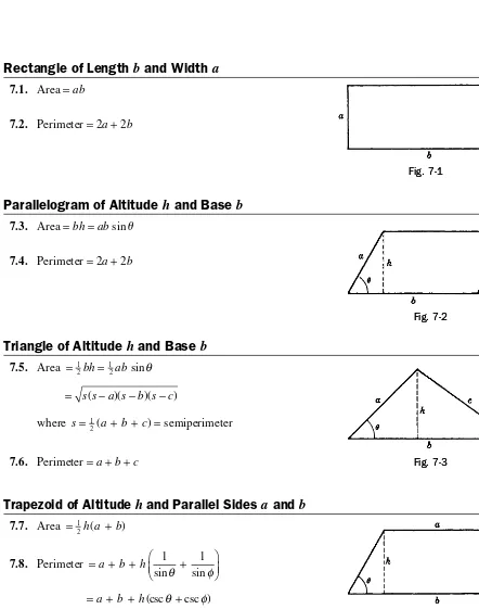
Rectangle of Length

b

and Width

a

7.1. Area =ab

7.2. Perimeter = 2a+ 2b

Parallelogram of Altitude

h

and Base

b

7.3. Area =bh=ab sin u

7.4. Perimeter = 2a+ 2b

Triangle of Altitude

h

and Base

b

7.5. Area = 1 =

2bh 12absinθ

= s s( −a s)( −b s)( −c) where s= 1 a+ +b c =

2( ) semiperimeter

7.6. Perimeter =a+b+c

Trapezoid of Altitude

h

and Parallel Sides

a

and

b

7.7. Area = 1₂h a( + b)

7.8. Perimeter = + +  +



 

a b h 1 1

sinθ sinφ

= + +a b h(cscθ +csc )φ

Fig. 7-1 Fig. 7-1

Fig. 7-2 Fig. 7-2

Fig. 7-3 Fig. 7-3

Fig. 7-4 Fig. 7-4

(29)

GEOMETRIC FORMULAS 17

Regular Polygon of

n

Sides Each of Length

b

7.9. Area = 1 =

4nb2 _n 14nb2

n n cotπ cos( / )_{sin( / )}_ππ

7.10. Perimeter =nb

Circle of Radius

r

7.11. Area =pr2

7.12. Perimeter = 2pr

Sector of Circle of Radius

r

7.13. Area = 1₂r2θ [q in radians]

7.14. Arc length s=rq

Radius of Circle Inscribed in a Triangle of Sides

a, b, c

7.15. r s s a s b s c

s

= ( − )( − )( − )

where s= 1₂(a+ +b c) = semiperimeter.

Radius of Circle Circumscribing a Triangle of Sides

a, b, c

7.16. R abc

s s a s b s c =

− − −

4 ( )( )( )

where s= 1₂(a+ +b c) = semiperimeter.

Fig. 7-5 Fig. 7-5

Fig. 7-6 Fig. 7-6

Fig. 7-7 Fig. 7-7

Fig. 7-8 Fig. 7-8

(30)

GEOMETRIC FORMULAS

Regular Polygon of

n

Sides Inscribed in Circle of Radius

r

7.17. Area = 12 2 = 12 2 °

2 360

nr

n nr n

sin π sin

7.18. Perimeter =2nr =2 180°

n nr n

sinπ sin

Regular Polygon of

n

Sides Circumscribing a Circle of Radius

r

7.19. Area =nr = °

n nr n

2_tanπ 2_tan180

7.20. Perimeter =2nr =2 180°

n nr n

tanπ tan

Segment of Circle of Radius

r

7.21. Area of shaded part = 1 − 2r2(θ sin )θ

Ellipse of Semi-major Axis

a

and Semi-minor Axis

b

7.22. Area =pab

7.23. Perimeter =4

∫

1− 2 2 0

2

a π/ k sin θ θd

=2 1 +

2 2 2

π (a b ) [approximately]

where k= a2−b a2/ . See Table 29 for numerical values.

Segment of a Parabola

7.24. Area = 2₃ab

7.25. Arc length ABC b a b

a

= 1 + +

2 2 2

2

16

8 ln

4_a _b2 16_a2

b

+ +

 

 

 

Fig. 7-10 Fig. 7-10

Fig. 7-11 Fig. 7-11

Fig. 7-12 Fig. 7-12

Fig. 7-13 Fig. 7-13

Fig. 7-14 Fig. 7-14

(31)

GEOMETRIC FORMULAS 19

Rectangular Parallelepiped of Length

a,

Height

b,

Width

c

7.26. Volume =abc

7.27. Surface area = 2(ab+ac+bc)

Parallelepiped of Cross-sectional Area

A

and Height

h

7.28. Volume =Ah=abc sinq

Sphere of Radius

r

7.29. Volume ₌ 4

3

πr

7.30. Surface area = 4πr2

Right Circular Cylinder of Radius

r

and Height

h

7.31. Volume =pr2h

7.32. Lateral surface area = 2prh

Circular Cylinder of Radius

r

and Slant Height

l

7.33. Volume =pr2_h₌_p_r2_l_sin_u

7.34. Lateral surface area ₌2π ₌ 2π ₌2

θ π θ

rl rh rh

sin csc

Fig. 7-15 Fig. 7-15

Fig. 7-16 Fig. 7-16

Fig. 7-17 Fig. 7-17

Fig. 7-18 Fig. 7-18

(32)

GEOMETRIC FORMULAS

20

Cylinder of Cross-sectional Area

A

and Slant Height

l

7.35. Volume =Ah=Al sinq

7.36. Lateral surface area =ph=pl sinq

Note that formulas 7.31 to 7.34 are special cases of formulas 7.35 and 7.36.

Right Circular Cone of Radius

r

and Height

h

7.37. Volume = 1₃πr h2

7.38. Lateral surface area =πr r2+ h2 = πrl

Pyramid of Base Area

A

and Height

h

7.39. Volume = 1₃ Ah

Spherical Cap of Radius

r

and Height

h

7.40. Volume (shaded in figure) =1₃πh2(3r−h)

7.41. Surface area = 2prh

Frustum of Right Circular Cone of Radii

a, b

and Height

h

7.42. Volume = 1₃πh a( 2+ab+b2)

7.43. Lateral surface area =π(a+b) h2+(b−a)2 =p(a+b)l

Fig. 7-20 Fig. 7-20

Fig. 7-21 Fig. 7-21

Fig. 7-22 Fig. 7-22

Fig. 7-23 Fig. 7-23

(33)

GEOMETRIC FORMULAS 21

Spherical Triangle of Angles

A, B, C

on Sphere of Radius

r

7.44. Area of triangle ABC= (A+B+C−p)r2

Torus of Inner Radius

a

and Outer Radius

b

7.45. Volume = 1 + −

4π2(a b b)( a)2 7.46. Surface area =p2₍_b2₋_a2₎

Ellipsoid of Semi-axes

a, b, c

7.47. Volume = 4 3πabc

Paraboloid of Revolution

7.48. Volume = 1₂πb a2

Fig. 7-25 Fig. 7-25

Fig. 7-26 Fig. 7-26

Fig. 7-27 Fig. 7-27

(34)

8

FORMULAS from PLANE ANALYTIC

GEOMETRY

Distance

d

Between Two Points

P

₁

(

x

₁

,

y

₁

)

and

P

₂

(

x

₂

,

y

₂

)

8.1. d= (x₂−x₁)2+ (y −y)

2 1 2

Slope

m

of Line Joining Two Points

P

₁

(

x

₁

,

y

₁

)

and

P

₂

(

x

₂

,

y

₂

)

8.2. m y y

x x

= −

− =

2 1

tanθ

Equation of Line Joining Two Points

P

₁

(

x

₁

,

y

₁

)

and

P

₂

(

x

₂

,

y

₂

)

8.3. y y

x x

y y

x x m y y m x x

−

− =

−

− = − = −

1

2 1

1 1

or ( )

8.4. y=mx+b

where b y mx x y x y x x

= − = −

−

1 1

2 1 1 2

2 1

is the intercept on the y axis,i.e., the yintercept.

Equation of Line in Terms of

x

Intercept

a

≠

0

and

y

Intercept

b

≠

0

8.5. x

a y b

+ =1

Fig. 8-1 Fig. 8-1

Fig. 8-2 Fig. 8-2

(35)

23

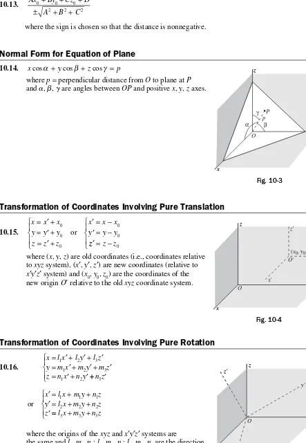
Normal Form for Equation of Line

8.6. xcos a+y sin a=p

where p= perpendicular distance from origin O to line and a= angle of inclination of perpendicular

with positive x axis.

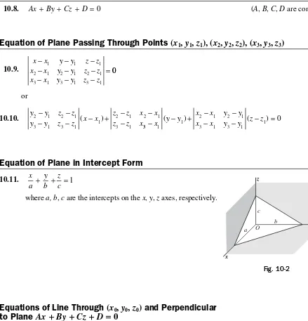
General Equation of Line

8.7. Ax+By+C= 0

Distance from Point

(

x

₁

, y

₁

)

to Line

Ax

+

By

+

C

=

₀

8.8. Ax By C

A B

1 1

2 2

+ +

± +

where the sign is chosen so that the distance is nonnegative.

Angle

x

Between Two Lines Having Slopes

m

₁

and

m

₂

8.9. tanψ = −

+

m m

m m

2 1

1 2

1

Lines are parallel or coincident if and only if m₁=m₂. Lines are perpendicular if and only if m₂=−1/m₁.

Area of Triangle with Vertices at

(

x

₁

,

y

₁

), (

x

₂

,

y

₂

), (

x

₃

,

y

₃

)

8.10. Area = ±1

2

1 1 1

1 1

2 2

3 3

x y x y x y

= ±1₂(x y1 2 + y x1 3 + y x3 2 − y x2 3 − y x1 2 − x y1 3)

where the sign is chosen so that the area is nonnegative. If the area is zero, the points all lie on a line.

Fig. 8-3 Fig. 8-3

Fig. 8-4 Fig. 8-4

Fig. 8-5 Fig. 8-5

(36)

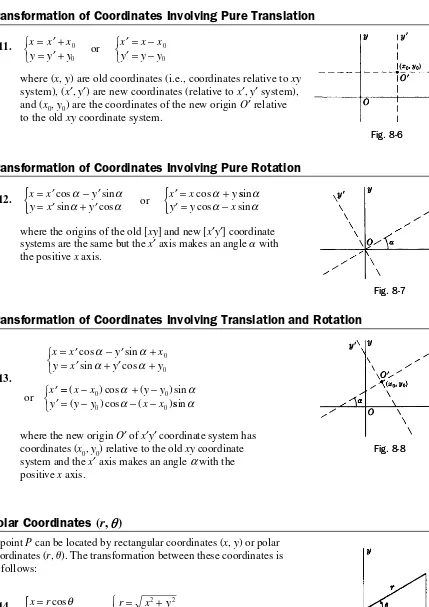
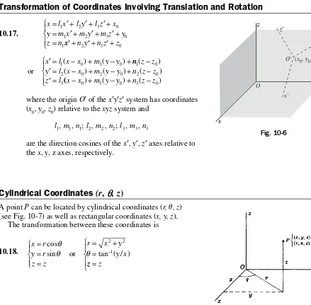
Transformation of Coordinates Involving Pure Translation

8.11. x x x

y y y

x x x y y y = ′ +

= ′ +   

′ = − ′ = −   

0

or

where (x, y) are old coordinates (i.e., coordinates relative to xy system), (x′, y′) are new coordinates (relative to x′, y′ system), and (x₀, y₀) are the coordinates of the new origin O′ relative to the old xy coordinate system.

Transformation of Coordinates Involving Pure Rotation

8.12. x x y

y x y

x x y

= ′ − ′

= ′ + ′

{

cos sin ′ = +

sin cos

cos

α α

α

or ssin

cos sin

α

α α

′ = −

{

y y x

where the origins of the old [xy] and new [x′y′] coordinate systems are the same but the x′ axis makes an angle a with the positive x axis.

Transformation of Coordinates Involving Translation and Rotation

8.13.

x x y x

y x y y

x

= ′ − ′ +

= ′ + ′ +

   ′

cos sin sin cos

α α

α α 00

or == − + −

′ = − − −

( ) cos ( )sin ( ) cos ( )

x x y y

y y y x x

0 0

α α

α ssinα

  

where the new origin O′ of x′y′ coordinate system has coordinates (x₀, y₀) relative to the old xy coordinate system and the x′ axis makes an angle a with the

positive x axis.

Polar Coordinates

(

r

,

p

)

A point P can be located by rectangular coordinates (x, y) or polar coordinates (r, u). The transformation between these coordinates is as follows:

8.14. x r

y r

r x y

y x =

=

{

= +

=  

 −

cos

sin _{tan ( / )}

θ

θ or _θ

2 2

1

Fig. 8-6 Fig. 8-6

Fig. 8-7 Fig. 8-7

Fig. 8-8 Fig. 8-8

Fig. 8-9 Fig. 8-9

(37)

25

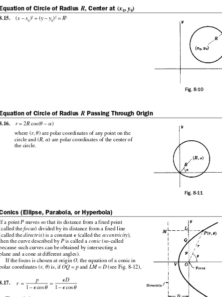
Equation of Circle of Radius

R

,

Center at

(

x

₀

,

y

₀

)

8.15. (x−x₀)2₊₍_y₋_y

0)2=R2

Equation of Circle of Radius

R

Passing Through Origin

8.16. r= 2R cos(u−a)

where (r, u) are polar coordinates of any point on the circle and (R, a) are polar coordinates of the center of the circle.

Conics (Ellipse, Parabola, or Hyperbola)

If a point P moves so that its distance from a fixed point (called the focus) divided by its distance from a fixed line (called the directrix) is a constant ⑀ (called the eccentricity),

then the curve described by P is called a conic (so-called because such curves can be obtained by intersecting a plane and a cone at different angles).

If the focus is chosen at origin O, the equation of a conic in polar coordinates (r, u) is, if OQ=p and LM=D (see Fig. 8-12),

8.17. r = p D

− = −

1 ⑀ 1

⑀ ⑀ cosθ cosθ

The conic is

(i) an ellipse if ⑀< 1

(ii) a parabola if ⑀= 1

(iii) a hyperbola if ⑀> 1

Fig. 8-10 Fig. 8-10

Fig. 8-11 Fig. 8-11

Fig. 8-12 Fig. 8-12

(38)

26

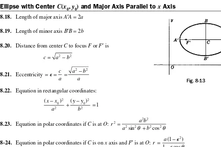
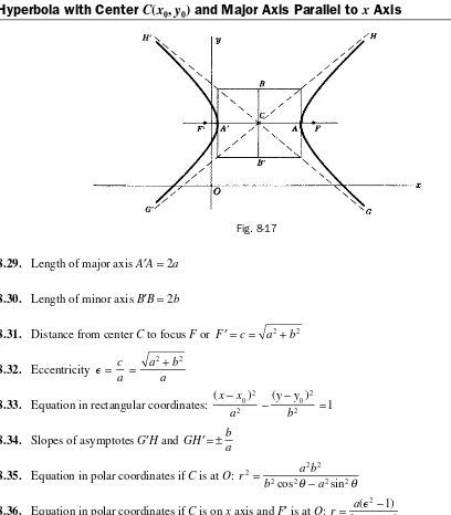
Ellipse with Center

C

(

x

₀

,

y

₀

)

and Major Axis Parallel to

x

Axis

8.18. Length of major axis A′A= 2a

8.19. Length of minor axis B′B= 2b

8.20. Distance from center C to focus F or F′ is c= a2 −b2

8.21. Eccentricity = =⑀ c = −

a

a b

a

2 2

8.22. Equation in rectangular coordinates:

(x x ) ( ) a

y y b −

+ − =

0 2 2

0 2

2 1

8.23. Equation in polar coordinates if C is at O: r a b

a b

2 2 2

2 2 2 2

=

+

sin θ cos θ

8-24. Equation in polar coordinates if C is on x axis and F′ is at O: r = a − −

( ) cos 1 1

2

⑀

⑀ θ

8.25. If P is any point on the ellipse, PF+PF′ = 2a

If the major axis is parallel to the y axis, interchange x and y in the above or replace u by 1₂π θ− (or 90° −u).

Parabola with Axis Parallel to

x

Axis

If vertex is at A (x₀,y₀) and the distance from A to focus F is a > 0, the equation of the parabola is

8.26. (y−y₀)2= 4a(x−x₀) if parabola opens to right (Fig. 8-14)

8.27. (y−y₀)2= −4a(x−x₀) if parabola opens to left (Fig. 8-15) If focus is at the origin (Fig. 8-16), the equation in polar coordinates is

8.28. r = a

−

2 1 cosθ

Fig. 8-13 Fig. 8-13

Fig. 8-14 Fig. 8-15 Fig. 8-16

FORMULAS FROM PLANE ANALYTIC GEOMETRY

(39)

27

Hyperbola with Center

C

(

x

₀

,

y

₀

)

and Major Axis Parallel to

x

Axis

Fig. 8-17

8.29. Length of major axis A′A= 2a

8.30. Length of minor axis B′B= 2b

8.31. Distance from center C to focus F or F′ = =c a2+b2

8.32. Eccentricity ⑀ = c = + a

a b

a

2 2

8.33. Equation in rectangular coordinates: (x x ) ( )

a

y y b −

− − =

0 2

2

0 2

2 1

8.34. Slopes of asymptotes G′H and GH b a ′= ±

8.35. Equation in polar coordinates if C is at O: r a b

b a

2 2 2

2 2 2 2

=

−

cos θ sin θ

8.36. Equation in polar coordinates if C is on x axis and F′ is at O: r= a − −

( ) cos ⑀

⑀

2 ₁

1 θ

8.37. If P is any point on the hyperbola, PF−PF′=±2a (depending on branch)

If the major axis is parallel to the y axis, interchange x and y in the above or replace u by 1 2π θ−

(or 90°−u).

(40)

Lemniscate

9.1. Equation in polar coordinates:

r2=a2 cos 2u

(x2+y2)2=a2(x2−y2)

9.3. Angle between AB′ or A′B and x axis = 45°

9.4. Area of one loop =a2

Cycloid

9.5. Equations in parametric form:

x a y a

= −

{

( sin ) ( cos )

φ φ

φ

1

9.6. Area of one arch = 3πa2

9.7. Arc length of one arch = 8a

This is a curve described by a point P on a circle of radius a rolling along x axis.

Hypocycloid with Four Cusps

x2/3+y2/3 =a2/3

9.9. Equations in parametric form:

x a y a = =   

cos sin

3

θ θ

9.10. Area bounded by curve ₌ 3 8πa2 9.11. Arc length of entire curve = 6a

This is a curve described by a point P on a circle of radius a/4 as it rolls on the inside of a circle of radius a.

Fig. 9-1 Fig. 9-1

Fig. 9-2 Fig. 9-2

Fig. 9-3 Fig. 9-3

9

SPECIAL PLANE CURVES

(41)

29

Cardioid

9.12. Equation: r= 2a(1 + cos u)

9.13. Area bounded by curve = 6pa2

9.14. Arc length of curve = 16a

This is the curve described by a point P of a circle of radius a as it rolls on the outside of a fixed circle of radius a. The curve is also a special case of the limacon of Pascal (see 9.32).

Catenary

9.15. Equation: y a e e a x

a

x a x a

= + − =

2 ( / / ) cos h

This is the curve in which a heavy uniform chain would hang if suspended vertically from fixed points A and B.

Three-Leaved Rose

9.16. Equation: r=a cos 3u

The equation r=a sin 3u is a similar curve obtained by rotating the curve of Fig. 9-6 counterclockwise through 30°

or p/6 radians.

In general, r=a cos nu or r=a sin nu has n leaves if n is odd.

Four-Leaved Rose

9.17. Equation: r=a cos 2u

The equation r=a sin 2u is a similar curve obtained by rotating the curve of Fig. 9-7 counterclockwise through 45°

or p/4 radians.

In general, r=a cos nu or r=asin nu has 2n leaves if n is even.

Fig. 9-4 Fig. 9-4

Fig. 9-5 Fig. 9-5

Fig. 9-6 Fig. 9-6

Fig. 9-7 Fig. 9-7

(42)

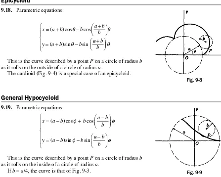
Epicycloid

9.18. Parametric equations:

x a b b a b

b

y a b b

= + − _ + _

= + −

( )cos cos

( )sin sin

θ θ

θ aa b

b +    

 

 

 θ

This is the curve described by a point P on a circle of radius b as it rolls on the outside of a circle of radius a.

The cardioid (Fig. 9-4) is a special case of an epicycloid.

General Hypocycloid

x a b b a b

b

y a b b

= − +  −

  

= − −

( ) cos cos

( )sin sin

φ φ

φ aa b

b −  

  

  

 

 φ

This is the curve described by a point P on a circle of radius b as it rolls on the inside of a circle of radius a.

If b=a/4, the curve is that of Fig. 9-3.

Trochoid

9.20. Parametric equations: x a b

y a b

= −

{

φ φ φ

sin cos

This is the curve described by a point P at distance b from the center of a circle of radius a as the circle rolls on the x axis.

If b < a, the curve is as shown in Fig. 9-10 and is called a curtate cycloid. If b > a, the curve is as shown in Fig. 9-11 and is called a prolate cycloid. If b=a, the curve is the cycloid of Fig. 9-2.

Fig. 9-8 Fig. 9-8

Fig. 9-9 Fig. 9-9

Fig. 9-11 Fig. 9-10

(43)

31

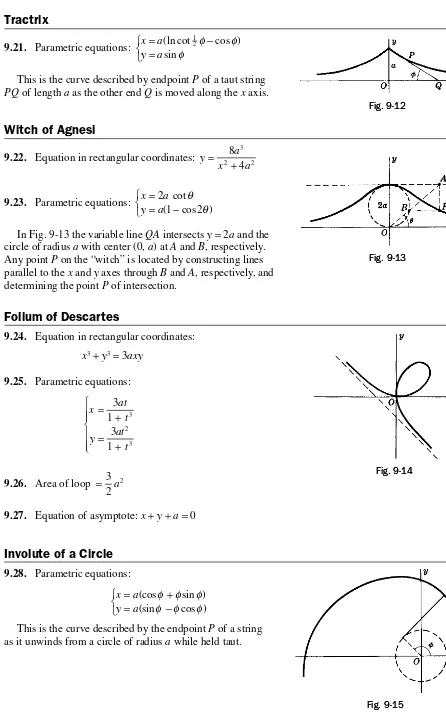
Tractrix

9.21. Parametric equations: x a

y a

= −

=   

( cot cos ) sin

ln 1

2φ φ

φ

This is the curve described by endpoint P of a taut string PQ of length a as the other end Q is moved along the x axis.

Witch of Agnesi

9.22. Equation in rectangular coordinates: y a

x a

= +

8 4

3

2 2

9.23. Parametric equations: x a

y a =

= −

  

2

1 2

cot ( cos )

θ θ

In Fig. 9-13 the variable line QA intersects y= 2a and the circle of radius a with center (0, a) at A and B, respectively. Any point P on the “witch” is located by constructing lines parallel to the x and y axes through B and A, respectively, and determining the point P of intersection.

Folium of Descartes

x3₊_y3₌₃_axy

x at

t y at

t =

+ =

+ 

 

  

3 1

3

2

3

9.26. Area of loop = 3

2a2

9.27. Equation of asymptote: x+y+a= 0

Involute of a Circle

x a y a

= +

= −

  

(cos sin ) (sin cos )

φ φ φ

This is the curve described by the endpoint P of a string as it unwinds from a circle of radius a while held taut.

Fig. 9-12 Fig. 9-12

Fig. 9-13 Fig. 9-13

Fig. 9-14 Fig. 9-14

Fig. 9-15 Fig. 9-15

(44)

32

Evolute of an Ellipse

(ax)2/3₊₍_by₎2/3₌₍_a2₋_b2₎2/3

ax a b by a b

= −

  

( ) cos ( )sin

2 2 3

θ θ

This curve is the envelope of the normals to the ellipse x2_/_a2₊_y2_/_b2₌_{1 shown dashed in Fig. 9-16.}

Ovals of Cassini

9.31. Polar equation: r4₊_a4₋₂_a2_r2_{cos 2}_u₌_b4

This is the curve described by a point P such that the product of its distance from two fixed points (distance 2a apart) is a constant b2_.

The curve is as in Fig. 9-17 or Fig. 9-18 according as b < a or b > a, respectively. If b=a, the curve is a lemniscate (Fig. 9-1).

Fig. 9-17 Fig. 9-18

Limacon of Pascal

9.32. Polar equation: r=b+a cos u

Let OQ be a line joining origin O to any point Q on a circle of diameter a passing through O. Then the curve is the locus of all points P such that PQ=b.

The curve is as in Fig. 9-19 or Fig. 9-20 according as 2a > b > a or b < a, respectively. If b=a, the curve is a cardioid (Fig. 9-4). If b⭌2 ,a the curve is convex.

Fig. 9-19 Fig. 9-20

Fig. 9-16 Fig. 9-16

(45)

33

Cissoid of Diocles

y x

a x

2 2

2

= −

x a

y a

= =   



2 2

2

3

sin sin cos

θ θ θ

This is the curve described by a point P such that the distance OP= distance RS. It is used in the problem of duplication of a cube, i.e., finding the side of a cube which has twice the volume of a given cube.

Spiral of Archimedes

9.35. Polar equation: r=au

Fig. 9-21 Fig. 9-21

Fig. 9-22 Fig. 9-22

(46)

Distance

d

Between Two Points

P

1

(

x

1

,

y

1

,

z

1

)

and

P

2

(

x

2

,

y

2

,

z

2

)

10.1. d= (x₂−x₁)2 + (y₂−y₁)2+ (z₂−z₁)2

Direction Cosines of Line Joining Points

P

1

(

x

1

,

y

1

,

z

1

)

and

P

2

(

x

2

,

y

2

,

z

2

)

10.2. l x x

d m

y y

d n

z z d = cosα = 2 − 1, =cosβ = 2 − 1, =cosγ = 2 − 1

where a, b, g are the angles that line P₁P₂ makes with the positive x, y, z axes, respectively, and d is given by 10.1 (see Fig. 10-1).

Relationship Between Direction Cosines

10.3. cos2α+cos2β + cos2γ =1 or l2+m2+n2 =1

Direction Numbers

Numbers L, M, N, which are proportional to the direction cosines l, m, n, are called direction numbers. The relationship between them is given by

10.4. l L

L M N m

M

L M N n

N

L M N

=

+ + = + + = + +

2 2 2 , 2 2 2 , 2 2 2

Equations of Line Joining

P

1

(

x

1

,

y

1

Mathematical Handbook of Formulas and Tables