CHAPTER IV
RESEARCH FINDING AND DISCUSSION
In this chapter, the writer presents the data which had been collected from the research in the field of study. The data are the result of pre-test experiment and control class, the result of post-test experiment and control class, result of data analysis, interpretation, and discussion.
A.Data Presentation
The Pre-test and Post-test at the experiment class had been conducted on July, 30th 2015(Thursday, at time 08.00-09.20) for Pre-test and August, 21st 2015 (Friday, at time 07.20–08.40) for Post- test in class VIII C of MTs Muslimat Nu Palangka Raya with the number of student was 36 students. Then the control class had been conducted on August, 4th 2015(Tuesday, at time 06.30–08.00) for Pre-test and August, 1st 2015 (Tuesday, at time 06.30–08.00) for Post- test in the class VIII A of MTs Muslimat Nu Palangka Raya with the number of student was 36 students.
In this chapter, the writer presents the obtained data of the students’ writing score, experiment class who was taught with picture series and control class who was taught without picture series.
1. Distribution of the Pre-Test Scores of the Experiment Class
Table 4.1 The Description of the Pre-Test Scores of the Experiment Class
NO STUDENT CODE SCORE
1 E1 61
2 E2 65
3 E3 70
4 E4 60
5 E5 70
6 E6 61
7 E7 66
8 E8 74
9 E9 78
10 E10 78
11 E11 65
12 E12 70
13 E13 65
14 E14 70
15 E15 66
16 E16 70
17 E17 65
18 E18 54
19 E19 58
20 E20 56
21 E21 54
22 E22 70
23 E23 60
24 E24 70
25 E25 79
26 E26 75
27 E27 54
28 E28 61
29 E29 63
30 E30 58
31 E31 69
32 E32 58
33 E33 64
34 E34 60
35 E35 65
Table 4.1 highlights that the student’s highest score is 79 and the student’s lowest score is 54. To determines the range of score, the class interval, and the interval temporary the writer calculates using formula as follows:
The Highest Score (H) = 79 The Lowest Score (L) = 54 The Range of Score (R) = H - L
= 79 - 54 = 25
The Class Interval (K) = 1+ 3.3 log n = 1+ 3.3 log 36 = 1+ 3.3 (1.56) = 1+ 5.148 = 6.148 = 6
Interval of Temporary (I) = 4.16667 4 5 6
25
or K
R
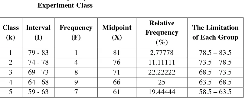
So, the range of score is 25, the class interval is 6, and interval of temporary is 5. Then, it is presented using frequency distribution in the following table: Table 4.2 The Frequency Distribution of the Pre-Test Score of the
Experiment Class
Class (k)
Interval (I)
Frequency (F)
Midpoint (X)
Relative Frequency
(%)
The Limitation of Each Group
1 79 - 83 1 81 2.77778 78.5 – 83.5
2 74 - 78 4 76 11.11111 73.5 – 78.5
3 69 - 73 8 71 22.22222 68.5 – 73.5
4 64 - 68 9 66 25 63.5 – 68.5
6 54 - 58 7 56 19.44444 53.5 – 58.5
TOTAL 36 100
Figure 4.1. The Frequency Distribution of the Pre-Test Score of the Experiment Class
Figure 4.1 shows that most of the students got score 63.5-68.5. It is proved that there are 9 students which is the greatest of number but their score are still below standard value. Whereas the lowest of number in the score 78.5-83.5 which is only 1 student. The students’ score which pass the standard value (67) are 23 students and there are 13 students whose score are below the standard value.
The next step, the writer tabulates the scores into the table for the calculation of mean, median, and modus as follows:
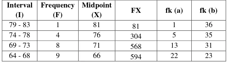
Table 4.3 The Calculation of Mean, Median, and Modus of the Pre-Test Scores of the Experiment Class
Interval
The Limitation of Each Group
59 - 63 7 61 427 29 14
54 - 58 7 56 392 36 7
TOTAL 36 2366
a. Mean
X = 𝑓𝑋 𝑁
=
2366
36
= 65.72222 b. Median
Me = l + i
1 2𝑛−𝑓𝑘𝑏
𝑓𝑖
= 63.5 + 5 1
2 36−14 9
= 63.5 + 5 0.44444 = 63.5 + (2.2222) = 65.7222
c. Modus
Mo = l + 𝑓𝑎
𝑓𝑎+𝑓𝑏
𝑖
= 63.5 + 8
8+7 5
= 63.5 + 0.53333 5 = 63.5 + 2.66665 = 66.16665
The last step, the writer tabulates the scores into the table for the calculation of standard deviation and the standard error as follows:
Table 4.4 The Calculation of the Standard Deviation and the Standard Error of the Pre-Test Scores of the Experiment Class
Interval
a. Standart Deviation
b. Standard Error
9161 . 5
8662 . 6
1 SEM
16059 . 1 1
SEM
The result of calculation reports that the standard deviation of pre test score of experiment class is 6.8662 and the standard error of pre test score of experiment class is 1.16059.
The next step, the writer calculates the scores of the pre test in experiment class using SPSS as follows:
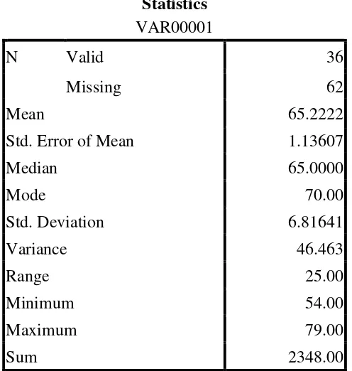
Table 4.5 The Table of Calculation of the Pre-Test Scores of the Experiment Class Using SPSS 16.0 Program
Statistics VAR00001
N Valid 36
Missing 62
Mean 65.2222
Std. Error of Mean 1.13607
Median 65.0000
Mode 70.00
Std. Deviation 6.81641
Variance 46.463
Range 25.00
Minimum 54.00
Maximum 79.00
2. Distribution of the Pre-Test of the Control Class
The pre test scores of the control class are presented in the following table. Table 4.6 The Description of the Pre-Test Scores of the Control Class
NO STUDENT CODE SCORE
1 C1 70
2 C2 63
3 C3 74
4 C4 73
5 C5 65
6 C6 65
7 C7 70
8 C8 74
9 C9 60
10 C10 65
11 C11 58
12 C12 58
13 C13 64
14 C14 73
15 C15 61
16 C16 65
17 C17 70
18 C18 66
19 C19 60
20 C20 56
21 C21 56
22 C22 56
23 C23 65
24 C24 70
25 C25 74
26 C26 60
27 C27 65
28 C28 65
29 C29 64
30 C30 63
31 C31 54
32 C32 61
33 C33 65
34 C34 70
35 C35 66
Table 4.6 highlights that the student’s highest score is 74 and the student’s lowest score is 54. To determines the range of score, the class interval, and the interval temporary the writer calculates using formula as follows:
The Highest Score (H) = 74 The Lowest Score (L) = 54 The Range of Score (R) = H - L
= 74 - 54 = 20
The Class Interval (K) = 1+ 3.3 log n = 1+ 3.3 log 36 = 1+ 3.3 (1.56) = 1+ 5.148 = 6.148 = 6
Interval of Temporary (I) = 3.33333 3 4 6
20
or K
R
So, the range of score is 20, the class interval is 6, and interval of temporary is 4. Then, it is presented using frequency distribution in the following table: Table 4.7 The Frequency Distribution of the Pre-Test Score of the Control
Class
Class (k)
Interval (I)
Frequency (F)
Midpoint (X)
Relative Frequency (%)
The Limitation of Each Group
1 74 - 77 3 75.5 8,333333 73.5 – 77.5
2 70 - 73 7 71.5 19,44444 69.5 – 73.5
3 66 - 69 2 67.5 5,555556 65.5 – 69.5
4 62 - 65 12 63.5 33,33333 61.5 – 65.5
6 54 - 57 4 55.5 11,11111 53.5 – 57.5
TOTAL 36 100
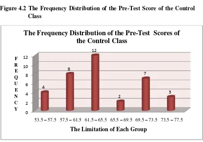
Figure 4.2 The Frequency Distribution of the Pre-Test Score of the Control Class
Figure 4.2 shows that most of the students got score 61.5-65.5. It is proved that there are 12 students which is the greatest of number but their score are still below standard value (67). Whereas the lowest of number in the score 65.5-69.5 which is only 2 students and both score are still below standard value (67). The
students’ score which pass the standard value (67) are 10 students and there are 26 students whose score are below the standard value.
The next step, the writer tabulates the score into the table for the calculation of mean, median, and modus as follows:
0 2 4 6 8 10 12
53.5 –57.5 57.5 –61.5 61.5 –65.5 65.5 –69.5 69.5 –73.5 73.5 –77.5 4
8
12
2
7
3
F R E Q U E N C Y
The Limitation of Each Group
Table 4.8 The Calculation of Mean, Median, and Modus of the Pre-Test Scores of the Control Class
Interval (I)
Frequency (F)
Midpoint
(X) FX fk (a) fk (b)
74 - 77 3 75.5 226,5 3 36
70 - 73 7 71.5 500,5 10 33
66 - 69 2 67.5 135 12 26
62 - 65 12 63.5 762 24 24
58 - 61 8 59.5 476 32 12
54 - 57 4 55.5 222 36 4
TOTAL 36 2322
a. Mean
X = 𝑓𝑋 𝑁
=
2322
36
= 64.5 b. Median
Me = 𝑙+𝑖
1 2𝑛−𝑓𝑘𝑏
𝑓𝑖
= 61.5 + 4 1
2 36−12 12
= 61.5 + 4 0.5 = 61.5 + 2 = 63.5 c. Modus
Mo = l + 𝑓𝑎 𝑓𝑎+𝑓𝑏
𝑖
= 61.5 + 2
= 61.5 + 0.2 4 = 61.5 + 0.8 = 62.3
From the calculation, the mean score is 64.5, median score is 63.5, and modus score is 62.3 of the pre-test of the control class.
The last step, the writer tabulates the scores into the table for the calculation of standard deviation and the standard error as follows:
Table 4.9 The Calculation of the Standard Deviation and the Standard Error of the Pre-Test Scores of the Control Class
Interval
a. Standard Deviation
b. Standard Error score of control class is 5.91604 and the standard error of pre test score of control class is 0.99999.
The next step, the writer calculates the scores of pre-test in control class using SPSS as follows:
Table 4.10 The Table of Calculation of the Pre-Test Scores of the Control Class Using SPSS 16.0 Program
Statistics
Median 65.0000
Mode 65.00
Std. Deviation 5.59308
Variance 31.283
Range 20.00
Minimum 54.00
Maximum 74.00
3. Distribution of the Post-Test Scores of the Experiment Class
The post test scores of the experiment class are presented in the following table.
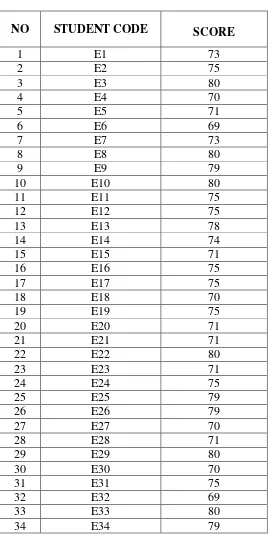
Table 4.11 The Description of the Post-Test Scores of the Experiment Class
NO STUDENT CODE SCORE
1 E1 73
2 E2 75
3 E3 80
4 E4 70
5 E5 71
6 E6 69
7 E7 73
8 E8 80
9 E9 79
10 E10 80
11 E11 75
12 E12 75
13 E13 78
14 E14 74
15 E15 71
16 E16 75
17 E17 75
18 E18 70
19 E19 75
20 E20 71
21 E21 71
22 E22 80
23 E23 71
24 E24 75
25 E25 79
26 E26 79
27 E27 70
28 E28 71
29 E29 80
30 E30 70
31 E31 75
32 E32 69
33 E33 80
35 E35 75
36 E36 73
Table 4.11 highlights that the student’s highest score is 88 and the student’s lowest score is 70. To determines the range of score, the class interval, and the interval temporary the writer calculates using formula as follows:
The Highest Score (H) = 80 The Lowest Score (L) = 69 The Range of Score (R) = H - L
= 80 - 69 = 11
The Class Interval (K) = 1+ 3.3 log n = 1+ 3.3 log 36 = 1+ 3.3 (1.56) = 1+ 5.148 = 6.148 = 6
Interval of Temporary (I) = 1.83333 2 6
11
K
R
So, the range of score is 11, the class interval is 6, and interval of temporary is 2. Then, it is presented using frequency distribution in the following table: Table 4.12 The Frequency Distribution of the Post-Test Score of the
Experiment Class
Class (k)
Interval (I)
Frequency (F)
Midpoint (X)
Relative Frequency (%)
The Limitation of Each Group
1 79 - 80 9 79.5 25 78.5 – 80.5
3 75 - 76 11 75.5 30,55556 74.5 – 76.5
4 73 - 74 2 73.5 5,555556 72.5 – 74.5
5 71 - 72 6 71.5 16,66667 70.5 – 72.5
6 69 - 70 7 69.5 19,44444 68.5 – 70.5
TOTAL 36 100
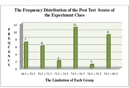
Figure 4.3. The Frequency Distribution of the Post-Test Scores of the Experiment Class
Figure 4.3 shows that most of the students got score 74.5-76.5. It is proved that there are 11 students which is the greatest of number. Whereas the lowest of number in the score 76.5-78.5 which is only 1 student. From the figure clarify that
all of the students’ score are pass the standard value (67).
The next step, the writer tabulates the score into the table for the calculation of mean, median, and modus as follows:
0 2 4 6 8 10 12
68.5 –70.5 70.5 –72.5 72.5 –74.5 74.5 –76.5 76.5 –78.5 78.5 –80.5 7
6
2
11
1
9 F
R E Q U E N C Y
The Limitation of Each Group
Table 4.13 The Calculation of Mean, Median, and Modus of the Post-Test Scores of the Experiment Class
Interval (I)
Frequency (F)
Midpoint
(X) FX fk (a) fk (b)
79 - 80 9 79.5 715.5 9 36
77 - 78 1 77.5 77.5 10 27
75 - 76 11 75.5 830.5 21 26
73 - 74 2 73.5 147 23 15
71 - 72 6 71.5 429 29 13
69 - 70 7 69.5 486.5 36 7
TOTAL 36 2686
a. Mean
X = 𝑓𝑋 𝑁
=
2686
36
= 74.61111 b. Median
Me = 𝑙+𝑖
1 2𝑛−𝑓𝑘𝑏
𝑓𝑖
= 74.5 + 2 1
2 36−13 11
= 74.5 + 2 0.45455 = 74.5 + 0.9091 = 75.4091 c. Modus
Mo = 𝑙 + 𝑓𝑎 𝑓𝑎+𝑓𝑏
𝑖
= 74.5 + 1
= 74.5 + 0.33333 x 2 = 74.5 + 0.66666
= 75.16666
From the calculation, the mean score is 74.61111, median score is 75.4091, and modus score is 75.16666 of the post-test of the experiment class.
The last step, the writer tabulates the scores into the table for the calculation of standard deviation and the standard error as follows:
Table 4.14 The Calculation of the Standard Deviation and the Standard Error of the Post-Test Scores of Experiment Class
Interval
a. Standard Deviation
63454 . 3 1
SD
b. Standard Error
1
The result of calculation reports that the standard deviation of the post-test score of the experiment class is 3.63454 and the standard error of post-test score of experiment class is 0.61435.
The next step, the writer calculates the scores of the post-test in experiment class using SPSS as follows:
Table 4.15 The Table of Calculation of the Post-Test Scores of the Experiment Class Using SPSS 16.0 Program
Statistics
Median 75.0000
Mode 75.00
Std. Deviation 3.90878
Variance 15.279
Range 11.00
Maximum 80.00
Sum 2685.00
4. Distribution of the Post-Test of the Control Class
The post test scores of the control class are presented in the following table.
Table 4.16 The Description of the Post-Test Scores of the Control Class
NO STUDENT CODE SCORE
1 C1 74
2 C2 74
3 C3 78
4 C4 78
5 C5 78
6 C6 65
7 C7 74
8 C8 78
9 C9 66
10 C10 71
11 C11 75
12 C12 70
13 C13 66
14 C14 70
15 C15 63
16 C16 74
17 C17 70
18 C18 70
19 C19 70
20 C20 61
21 C21 70
22 C22 61
23 C23 74
24 C24 74
25 C25 66
26 C26 71
27 C27 75
28 C28 74
30 C30 75
31 C31 78
32 C32 74
33 C33 70
34 C34 63
35 C35 74
36 C36 70
Table 4.16 highlights that the student’s highest score is 78 and the student’s lowest score is 61. To determines the range of score, the class interval, and the interval temporary the writer calculates using formula as follows:
The Highest Score (H) = 78 The Lowest Score (L) = 61 The Range of Score (R) = H - L
= 78 – 61 = 17 The Class Interval (K) = 1+ 3.3 log n
= 1+ 3.3 log 36 = 1+ 3.3 (1.56) = 1+ 5.148 = 6.148 = 6
Interval of Temporary (I) = 2.83333 2 3 6
17
or K
R
Table 4.17 The Frequency Distribution of the Post-Test Score of the Control
Figure 4.4 The Frequency Distribution of the Post-Test Score of the Control Class
Figure 4.4 shows that most of the students got score 72.5-75.5. It is proved that there are 13 students which is the greatest of number. Whereas the lowest of number in the score 66.5-69.5 which there is no students got that score. The
students’ score which pass the standard value (67) are 28 students and there are 8 0
The Limitation of Each Group
students whose score are below the standard value. It means that the most of students got score which pass the standard value (67).
The next step, the writer tabulates the score into the table for the calculation of mean, median, and modus as follows:
Table 4.18 The Calculation of Mean, Median, and Modus of the Post-Test Scores of the Control Class
Interval (I)
Frequency (F)
Midpoint
(X) FX fk (a) fk (b)
76 - 78 5 77 385 5 36
73 - 75 13 74 962 18 31
70 - 72 10 71 710 28 18
67 - 69 0 68 0 28 8
64 - 66 4 65 260 32 8
61 - 63 4 62 248 36 4
TOTAL 36 2565
a. Mean
X = 𝑓𝑋 𝑁
= 2565 36
= 71.25 b. Median
Me = 𝑙+𝑖
1 2𝑛−𝑓𝑘𝑏
𝑓𝑖
= 72.5 + 3 1
2 36−18 13
c. Modus modus score is 73.49999 of the post-test of the control class.
The last step, the writer tabulates the scores into the table for the calculation of standard deviation and the standard error as follows:
Table 4.19 The Calculation of the Standard Deviation and the Standard Error of the Post-Test Scores of the Control Class
Interval
a. Standard Deviation
2
b. Standard Error
1 control class is 0.77804.
The next step, the writer calculates the scores of the post-test in control class using SPSS as follows:
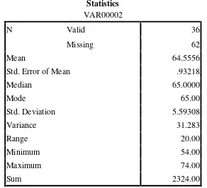
Table 4.20 The Table of Calculation of the Post-Test Scores of the Control Class Using SPSS 16.0 Program
Statistics VAR00002
N Valid 36
Missing 0
Std. Error of Mean .80966
Median 72.5000
Mode 74.00
Std. Deviation 4.85798
Variance 23.600
Range 17.00
Minimum 61.00
Maximum 78.00
Sum 2568.00
B.Result of Data Analysis
1. Testing of Normality and Homogeneity
The writer calculates the result of pre-test and post-test score of experiment and control class by using SPSS 16.0 program. It is used to know the normality of the data that is going to be analyzed whether both groups have normal distribution or not. Also, homogeneity is used to know whether experiment class and control class, that are decided, come from population that has relatively same variant or not.
a. Testing of Normality and Homogeneity of Pre-Test of Experiment and Control Class
Table 4.21 Testing of Normality One-Sample Kolmogorov-Smirnov Test
One-Sample Kolmogorov-Smirnov Test
VAR00001
N 72
Normal Parametersab
Mean 64.8889
Std. Deviation 6.19985
Most Extreme Differences
Absolute .109
Positive .109
Kolmogorov-Smirnov Z .929
Asymp. Sig. (2-tailed) .354
a. Test distribution is Normal. b. Calculated from data
Based on the calculation uses SPSS program, the asymptotic significant normality of experiment class and control class is 0.354. Then the normality both of class is consulted with table of Kolmogorov- Smirnov with the level of
significant 5% (α=0.05). Since asymptotic significant of experiment and
asymptotic significant of control= 0.354 ≥ α = 0.05. It can be concluded that the data distribution is normal.
Table 4.22 Testing Homogeneity Levene's Test of Equality of Error Variancesa
Test of Homogeneity of Variances Dependent variable: Achievement
Levene Statistic df1 df2 Sig.
1.374 1 70 .245
Based on the result of homogeneity test, the data are homogeneous if the significantvalue is higher than significant level α= 0.05. Table 4.22 proves that the
significantvalue (0.245) is higher than significant level α= 0.05, it can be concluded
b.Testing of Normality and Homogeneity for Post-Test of Experiment and Control Class
Table 4.23 Testing of Normality One-Sample Kolmogorov-Smirnov Test
One-Sample Kolmogorov-Smirnov Test
VAR00002
N 72
Normal Parametersab
Mean 72.9583
Std. Deviation 4.67368
Most Extreme Differences
Absolute .130
Positive .109
Negative -.130
Kolmogorov-Smirnov Z 1.102
Asymp. Sig. (2-tailed) .176
a. Test distribution is Normal. b.Calculated from data
Based on the calculation uses SPSS program, the asymptotic significant normality of experiment class and control class are 0.176. Then the normality both of class are consulted with table of Kolmogorov- Smirnov with the level of significant 5% (α=0.05). Since asymptotic significant of experiment and asymptotic significant of control= 0.176 ≥ α = 0.05. It can be concluded that the data distribution is normal.
Table 4.24 Testing of Homogeneity Levene's Test of Equality of Error Variancesa
Test of Homogeneity of Variances Dependent variable: Achievement
Levene Statistic df1 df2 Sig.
Based on the result of homogeneity test, the data are homogeneous if the significantvalue is higher than significant level α= 0.05. Table 4.24 proves that the
significantvalue (0.259) is higher than significant level α= 0.05, it can be concluded
that the data are homogeneous. It means that both of classes have same variants. 2. Testing Hypothesis
a. Testing Hypothesis Using T-test
The writer uses t-test statistical calculation with significant level of the the refusal null hypothesis α= 0.05. The writer uses manual calculation and SPSS 16.0. Program test the hypothesis using t-test statistical calculation. The criteria of Ha is accepted when tobseved > ttable, and Ho is refused when tobserved < ttable. The
result of testing hypothesis explained in the following table.
Table 4.25 The Standard Deviation and the Standard Error of X1 and X2
Variable The Standard Deviation The Standard Error
X1 3.63454 0.61435
X2 4.60299 0.77804
Where:
X1 = Experimental Class
X2 = Control Class
The table shows the result of the standard deviation calculation of X1 is
3.63454 and the result of the standard error mean calculation is 0.61435. The result of the standard deviation calculation of X2 is 4.60299 and the result of the
The next step, the writer calculates the standard error of the differences With the criteria:
If t-test (tobserved) ≥ ttable, it means Ha is accepted and H0 is rejected.
If t-test (tobserved) < ttable, it means Ha is rejected and H0 is accepted.
Then, the writer interprets the result of t-test. Previously, the writer accounts the degree of freedom (df) with the formula:
table
t
at df 70/60 at 5% significant level = 2.00The calculation above shows the result of t-test calculation as in the table follows:
Table 4.26 The Result of T-test
Variable tobserved
ttable
Df/db
5% 1%
X1- X2 3.390 2.00 2.66 70/60
Where:
X1 = Experimental Class
X2 = Control Class
tobserved = The calculated Value
ttable = The distribution of t value
df/db = Degree of Freedom
The result of hypothesis test calculation (Table 4.26) proves that the value of tobserved is higher than the value of ttable at the level of significant in 5% or 1%
b. Testing Hypothesis Using SPSS Program
The writer also applies SPSS 16.0 program to calculate t-test in testing hypothesis of the study which supports the result of manual calculation. The result of the test using SPSS 16.0 program can be seen as follows:
Table 4.27 The Calculation of T-test Using SPSS 16.0
Independent Samples Test
Levene's Test for Equality of
Variances t-test for Equality of Means
F Sig. t df
Table 4.27 reports that Ha is accepted. It is found that the result of tobserved
= 3.127 is higher than ttable = 2.00 in the significant level of 5% and 2.66 in the
significance level of 1%. It can be interpreted that alternative hypothesis (Ha) is
accepted. It means students who taught using picture series give significant effect
C.Interpretation
The hypothesis testing uses T-test to measures the significant effect of using Picture Series toward students’ writing score in recount text. Based on the manual calculation and SPSS 16.0 program of T-test the tobserved= 3.127 is
consulted with ttable with significant level 5% (2.00) and 1% (2.66) or 2.00
<3.127>2.66. It can be concluded that using Picture Series toward students’ writing score in recount text is significant.
The result of calculation proves that Ha stating there is significant effect of picture series toward writing score of the eighth graders of Muslimat Nu Palangka Raya is accepted and H0 stating there is no significant effect of picture series toward writing score of the eighth graders of Muslimat Nu Palangka Raya is rejected. It means, the students who taught with Picture Series have better writing score than the students who taught without Picture Series.
D.Discussion
The result of analysis shows that there is significant effect of using Picture Series toward writing score in recount text at the eighth graders of MTs Muslimat Nu Palangka Raya. The students who are taught using Picture Series get higher score in post-test with mean (74.61) than those students who are taught by conversional method with mean (71.25). Moreover, after the data calculates using T-test and it is found the tobserved is 3.390 and ttable 2.00. It means that tobserved > ttable.
writing score. It is proved by the value of tobserved is higher than ttable at 5% and 1%
significant level or 2.00<3.127 >2.66. This finding indicates that the alternative hypothesis stating that there is any significant effect of using Picture Series toward writing score of the eighth graders in writing recount text is accepted. On contrary, the null hypothesis is rejected.
From the observation of teaching learning process, it can be seen many
improvement from students’ side. In the pre-observation, many students seemed not to have motivation, they got boredom in writing class and they got difficulty to choose the words and to express their ideas. These behaviour started to change where teaching learning process had done well. The class condition was better than previous meeting. There several result of implementation of using Picture Series in writing recount text. First, based on in teaching learning process, the students understand what should they do and write when the researcher show the picture. The finding is suitable with Betty Morgan Bowen statement which had been explained in chapter II that a picture series is a number of related composites pictures linked to form a series or sequences. Hence, its main function is to tell a story or sequences of events. It means that from the picture series, learners will easier to understand the meaning of a word, sentence or event a paragraph after they see the picture itself.
to learn the material, in writing aspect for example. This finding is related to Francis which the statement in chapter II, he said that picture increase students’ motivation and provide useful practice material as well as test material.
Third, the implementation had done can build students’ interest in learning language through pictures. It is related to Hill statement which also had been explained in chapter II that picture has the advantages of being inexpensive, of being available in most situations. Fourth, picture series can solve the problems of writing,
1. Lack of Vocabulary: Picture series can promote many vocabularies for the
students.
2. Grammatical mistake: From the picture series the teacher can mention some action
verb and ask the students to make the sentence based on the words in past form.
3. Idea organization: Some students often think that it is hard to get an idea to build
their sentence. And here picture series contain of many actions that can be applied
as idea or to provoke the students in imagining something,
Based on statements above can stated using Picture Series gives effect on
Based on the research finding, also indicates students’ score in control class who taught by conversional teaching, also improved from Pre- test to Post- test. It is caused by familiar theme that applied in teaching writing recount text because it is based on their experiences. Also, the writer who asked the students made outline before writing the paragraph, it made the students easily to analyze the organization concerning orientation, events, and re-orientation of the story. It can be concluded that any factors also improve the students’ score on this study besides the effect of using picture series as media in teaching writing recount text such as based on their experiences, familiar theme and dictionary that they used to find new vocabulary. Teaching writing using Picture Series is more interesting and can help students to get the ideas. The students might be motivated to write their story chronologically. Also, they can enjoy.