A. Data Presentation - The effect of word wall toward students’ vocabulary score at the eight grade students of MTs Muslimat NU Palangka Raya - Digital Library IAIN Palangka Raya

(1)

CHAPTER IV

RESEARCH FINDING AND DISCUSSION

In this chapter, the writer presents the data which had been collected from the research in the field of study. The data are the result of pre-test experiment and control class, the result of post-test experiment and control class, result of data analysis, interpretation, and discussion. A.Data Presentation

The Pre-test and Post-test at the experiment class had been conducted on May, 20th 2016(Friday, at time 07.20-08.40 a.m) for Pre-test and April, 28th 2016 (Thursday, at time 08.00– 09.40 a.m) for Post- test in class VIII C of MTs Muslimat Nu Palangka Raya with the number of student was 39 students. Then the control class had been conducted on April, 26th 2016(Tuesday, at time 06.30–08.00 a.m) for Pre-test and May, 18th 2016 (Wednesday, at time 12.00–01.20 a.m) for Post- test in the class VIII A of MTs Muslimat Nu Palangka Raya with the number of student was 39 students.

In this chapter, the writer presents the obtained data of the students’ vocabulary score, experiment class who was taught with word wall and control class who was taught without word wall.

1. Distribution of the Pre-Test Scores of the Experiment Class

(2)

No Experiment Class

Students’ Code Score Grade

(3)

Based on the data above, it can be seen that the students’ highest score is 78 and the student’s lowest score is 53. To determine the range of score, the class interval, and interval of temporary, the writer calculated using formula as follows:

The highest score (H) : 78 Interval of temporary (I) =R

K = 25

6 = 4.16667 = 4 𝑜𝑟 5

So, the range of score is 25, the class interval is 6, and interval of temporary is 5. Then, it is presented using frequency distribution in the following table:

Table 4.2 The Frequency Distribution of the Pre-Test Score of the Experiment Class

(4)

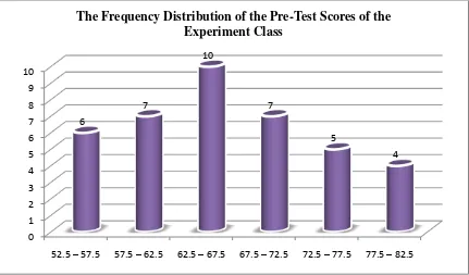
Figure 4.1. The Frequency Distribution of the Pre-Test Score of the Experiment Class

Figure 4.1 shows that most of the students got score 62.5-67.5. It is proved that there are 10 students which is the greatest of number but their score are still below standard value. Whereas the lowest of number in the score 77.5-82.5 which is only 4 student. The students’ score which pass the standard value (67) are 23 students and there are 13 students whose score are below the standard value.

The next step, the writer tabulates the scores into the table for the calculation of mean, median, and modus as follows:

Table 4.3 The Calculation of Mean, Median, and Modus of the Pre-Test Scores of the The Frequency Distribution of the Pre-Test Scores of the

(5)

69 – 73 8 71 568 16 31

64 – 68 9 66 594 25 23

59 – 63 7 61 427 32 14

55 - 58 7 56 392 39 7

TOTAL 39 2604

a. Mean

X ₌ 𝑓𝑋

𝑁

= 2585 39

= 66.28205

b. Median

Me = l + i 1 2 𝑛−𝑓𝑘𝑏

𝑓𝑖

= 62.5 + 4 1 2 39−6

10

= 62.5 + 4 1.35

= 62.5 +5.4 = 67.9 c. Modus

Mo ₌ l₊ 𝑓𝑎

𝑓𝑎+𝑓𝑏 𝑖

(6)

From the calculation, the mean score is 66.28205, median score is 69.25, and modus score is 65 of the pre-test of the experiment class.

The last step, the writer tabulates the scores into the table for the calculation of standard deviation and the standard error as follows:

Table 4.4 The Calculation of the Standard Deviation and the Standard Error of the Pre-Test Scores of the Experiment Class

(7)

1

The result of calculation reports that the standard deviation of pre test score of experiment class is 7.6994 and the standard error of pre test score of experiment class is 1.249

The next step, the writer calculates the scores of the pre test in experiment class using SPSS 18.0 as follows:

Table 4.5 The Table of calculation of The Pre-Test Scores of The Experiment Class Using SPSS 18.0 Program

Std. Deviation 6.955

Variance 48.366

Range 23

Minimum 61

Maximum 84

(8)

2. Distribution of the Pre-Test of the Control Class

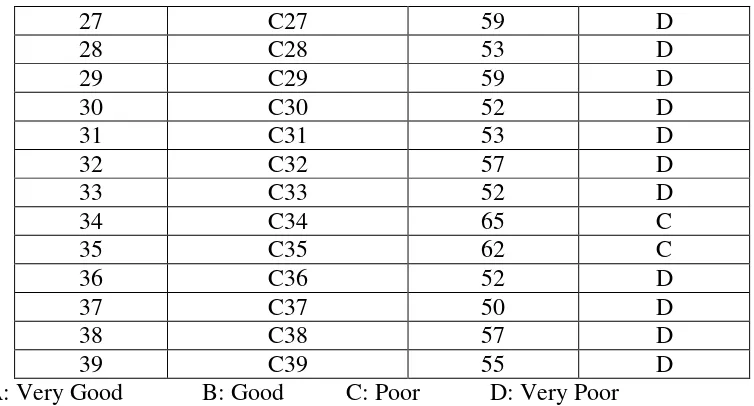
The pre test scores of the control class are presented in the following table. Table 4.6 The Description of the Pre-Test Scores of the Control Class

No Control Class

1 C01 60 C

2 C02 65 C

3 C03 59 D

4 C04 48 D

5 C05 67 C

6 C06 67 C

7 C07 48 D

8 C08 46 D

9 C09 48 D

10 C10 59 D

11 C11 65 C

12 C12 65 C

13 C13 48 D

14 C14 64 C

15 C15 65 C

16 C16 57 D

17 C17 48 D

18 C18 50 D

19 C19 64 C

20 C20 67 C

21 C21 52 D

22 C22 57 D

23 C23 57 D

24 C24 62 C

25 C25 70 B

(9)

27 C27 59 D

28 C28 53 D

29 C29 59 D

30 C30 52 D

31 C31 53 D

32 C32 57 D

33 C33 52 D

34 C34 65 C

35 C35 62 C

36 C36 52 D

37 C37 50 D

38 C38 57 D

39 C39 55 D

A: Very Good B: Good C: Poor D: Very Poor

Table 4.6 highlights that the student’s highest score is 70 and the student’s lowest score is 46. To determines the range of score, the class interval, and the interval temporary the writer calculates using formula as follows:

The Highest Score (H) = 70

The Lowest Score (L) = 46

The Range of Score (R) = H - L = 70 - 46 = 24

The Class Interval (K) = 1+ 3.3 log n = 1+ 3.3 log 39 = 1+ 3.3 (1.59) = 1+ 5.247 = 6.247 = 6

Interval of Temporary (I) = 4 6 24_



(10)

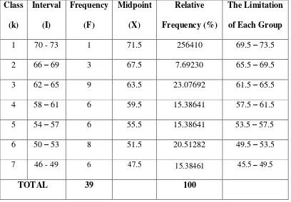
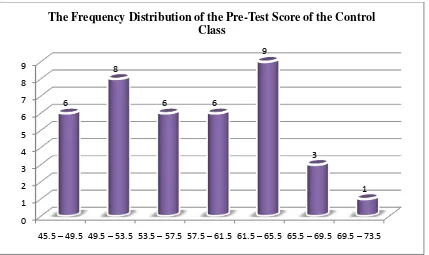
Table 4.7 The Frequency Distribution of the Pre-Test Score of the Control Class Class

(k)

Interval (I)

Frequency (F)

Midpoint (X)

Relative Frequency (%)

The Limitation of Each Group

1 70 - 73 1 71.5 256410 69.5 – 73.5

2 66 – 69 3 67.5 7.69230 65.5 – 69.5

3 62 – 65 9 63.5 23.07692 61.5 – 65.5 4 58 – 61 6 59.5 15.38641 57.5 – 61.5 5 54 – 57 6 55.5 15.38641 53.5 – 57.5 6 50 – 53 8 51.5 20.51282 49.5 – 53.5

7 46 - 49 6 47.5 _15.38461 45.5 – 49.5

TOTAL 39 100

(11)

Figure 4.2 shows that most of the students got score 61.5-65.5. It is proved that there are 9 students which is the greatest of number but their score are still below standard value (66). Whereas the lowest of number in the score 69.5-73.5 which is only 1 student and both score are still below standard value (66). The students’ score which pass the standard value (66) are 13 students and there are 14 students whose score are below the standard value.

The next step, the writer tabulates the score into the table for the calculation of mean, median, and modus as follows:

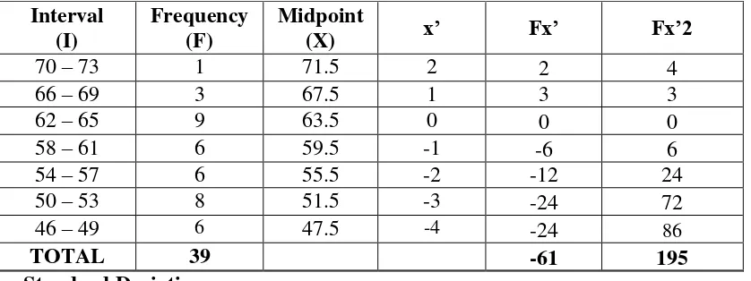
Table 4.8 The Calculation of Mean, Median, and Modus of the Pre-Test Scores of the Control Class

Midpoint

(X) FX fk (a) fk (b)

0 1 2 3 4 5 6 7 8 9

45.5 –49.5 49.5 –53.5 53.5 –57.5 57.5 –61.5 61.5 –65.5 65.5 –69.5 69.5 –73.5 6

8

6 6

9

3

1 The Frequency Distribution of the Pre-Test Score of the Control

(12)

70 – 73 1 71.5 71.5 1 39

66 – 69 3 67.5 202.5 4 38

62 – 65 9 63.5 571.5 13 35

58 – 61 6 59.5 357 19 26

54 – 57 6 55.5 333 25 20

50 – 53 8 51.5 412 33 14

46 – 49 6 47.5 285 39 6

TOTAL 39 2232.5

a. Mean

X ₌ 𝑓𝑋

𝑁

= 2232 .5 39

= 57.24358 b. Median

Me ₌𝑙₊𝑖

1 2𝑛−𝑓𝑘𝑏

𝑓𝑖

= 53.5 + 6 1 2 39−14

9

= 53.5 + 6 0.61111

= .53.5+ 3.66666 = 57.16666 c. Modus

Mo ₌l₊ 𝑓𝑎

𝑓𝑎+𝑓𝑏 𝑖

(13)

From the calculation, the mean score is 57.24358, median score is 65.16666, and modus score is 62.16666 of the pre-test of the control class.

Table 4.9 The Calculation of the Standard Deviation and the Standard Error of the Pre-Test Scores of the Control Class

(14)

𝑆𝐷2 = 6.39199 class is 6.39199 and the standard error of pre test score of control class is 1.0369.

The next step, the writer calculates the scores of pre-test in control class using SPSS 18.0 as follows:

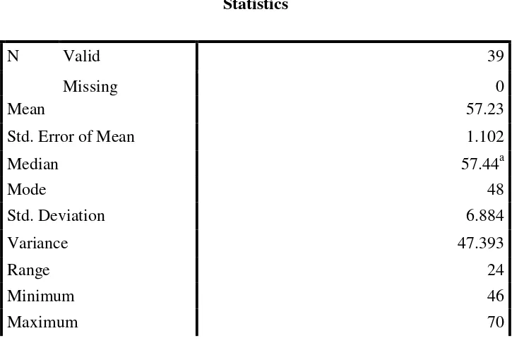
Table 4.10 The Table of Calculation of the Pre-Test Scores of the Control Class Using SPSS 18.0 Program

Variance 47.393

Range 24

Minimum 46

(15)

Sum 2232

3. Distribution of the Post-Test Scores of the Experiment Class

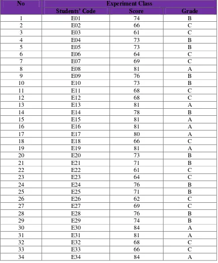
The post test scores of the experiment class are presented in the following table. Table 4.11 The Description of the Post-Test Scores of the Experiment Class

No Experiment Class

(16)

35 E35 61 C

36 E36 68 C

37 E37 83 A

38 E38 74 B

39 E39 76 B

Table 4.11 highlights that the student’s highest score is 84 and the student’s lowest score is 61. To determines the range of score, the class interval, and the interval temporary the writer calculates using formula as follows:

The Range of Score (R) = H - L = 84 - 61 = 23

The Class Interval (K) = 1+ 3.3 log n = 1+ 3.3 log 39 = 1+ 3.3 (1.59) = 1+ 5.247 = 6.247 = 6

Interval of Temporary (I) = 3.83333 3 6

23 _ _



K R

(17)

Class

Figure 4.2 shows that most of the students got score 72.5-76.5. It is proved that there are 11 students which is the greatest of number but their score are still below standard value (66). Whereas the higher of number in the score 80.5-84.5 which is 9 students and there are 13 students whose score are below the standard value.

0

(18)

(19)

= 72.5 + (0.61111)2 = 72.5 + 1.2222

= 73.72222

From the calculation, the mean score is 72.35897 , median score is 75.4545 , and modus score is 73.72222 of the post-test of the experiment class.

Table 4.14 The Calculation of the Standard Deviation and the Standard Error of the Post-Test Scores of Experiment Class

(20)

𝑆𝐷1 = 3.47054

b. Standard Error

1

1 1 1

 

N SD SEM

𝑆𝐸𝑀1 =

3.47054 39−1

𝑆𝐸𝑀1 =

3.47054 38

𝑆𝐸𝑀1 =

3.47054 6.164

𝑆𝐸𝑀1 = 0.56303

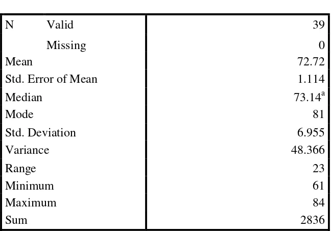
Table 4.15 The Table of the Calculation of Post-Test Scores of Experimant Class

Statistics

N Valid 39

Missing 0

Mean 72.72

Std. Error of Mean 1.114

Median 73.14a

Mode 81

Variance 48.366

Range 23

Minimum 61

Maximum 84

(21)

4. Distribution of the Post-Test of the Control Class

The post test scores of the control class are presented in the following table. Table 4.16 The Description of the Post-Test Scores of the Control class

(22)

33 C33 58 D

34 C34 65 C

35 C35 72 B

36 C36 60 C

37 C37 59 D

38 C38 65 C

39 C39 62 C

Table 4.16 highlights that the student’s highest score is 78 and the student’s lowest score is

56. To determines the range of score, the class interval, and the interval temporary the writer calculates using formula as follows:

The Range of Score (R) = H - L

= 78 – 56 = 22 The Class Interval (K) = 1+ 3.3 log n

= 1+ 3.3 log 39 = 1+ 3.3 (1.59) = 1+ 5.247 = 6.247 = 6

Interval of Temporary (I) = 3.66666 3 4 6

22

or K

R

 



So, the range of score is 22, the class interval is 6, and interval of temporary is 3.66666 Then, it is presented using frequency distribution in the following table:

(23)

Class

Figure 4.4 The Frequency Distribution of the Post-Test Score of the Control Class

Figure 4.4 shows that most of the students got score 61.5-65.5. It is proved that there are 12 students which is the greatest of number. The students’ score which pass the standard value (66) are 15 students and there are 8 students whose score are below the standard value. It means that the most of students got score which pass the standard value (66).

0

(24)

Table 4.18 The Calculation of Mean, Median, and Modus of the Post-Test Scores of the Control Class

Midpoint

(X) FX fk (a) fk (b)

75 – 78 1 76.5 76.5 1 39

71 – 74 4 72.5 290 5 38

67 – 70 5 68.5 342.5 10 34

63 – 66 3 64.5 193.5 13 29

59 – 62 12 60.5 762 25 26

55 – 58 11 56.5 621.5 36 14

51 – 54 3 52.5 157.5 39 3

TOTAL 39 2407.5

a. Mean

X ₌ 𝑓𝑋

𝑁

= 2407 .5 39

= 61.73076

b. Median

Me ₌𝑙₊𝑖

1 2𝑛−𝑓𝑘𝑏

𝑓𝑖

= 58.5 + 4 1 2 39−14

12

= 58.5 + 4 0.45834

= 58.5 + 1.83336 = 60.33336

(25)

Mo ₌l₊ 𝑓𝑎 score is 59.5 of the post-test of the control class.

Table 4.19 The Calculation of the Standard Deviation and the Standard Error of the Post-Test Scores of the Control Class

(26)

𝑆𝐷2 = 2

The result of calculation reports that the standard deviation of post-test score of control class is 3.11008 and the standard error of post-test score of control class is 0.50455.

(27)

Median 60.60a

Mode 58

Variance 39.968

Range 26

Minimum 52

Maximum 78

Sum 2415

5. Comparison Result of Pre Test and Post Test Score of Experiment Class

The comparison between pre test and post test score of experiment class were presented in table 4.20 as follow:

Tabel 4.20 The Comparison Pre Test and Post Test Score of Experiment Class

No Students

’ Code Pre Test Experiment Class Diff

Score

Grade Post Test

Score

Grade

1 E01 63 C 74 B 11

2 E02 62 C 66 C 4

3 E03 56 D 61 C 5

4 E04 59 D 73 B 14

5 E05 72 B 73 B 1

6 E06 57 D 64 C 7

7 E07 66 C 69 C 3

8 E08 59 D 81 A 12

9 E09 53 D 76 B 23

10 E10 69 C 73 B 4

11 E11 59 D 63 C 4

12 E12 57 D 68 C 11

13 E13 62 C 81 A 19

(28)

15 E15 60 C 81 A 21

16 E16 67 C 81 A 14

17 E17 72 D 80 A 8

18 E18 63 C 66 C 3

19 E19 60 C 81 A 21

20 E20 56 D 73 B 17

21 E21 63 C 71 B 8

22 E22 57 D 61 C 4

23 E23 62 C 64 C 2

24 E24 60 C 76 B 16

25 E25 72 B 71 B -1

26 E26 53 D 62 C 9

27 E27 69 C 69 C 0

28 E28 57 D 76 B 19

29 E29 67 C 74 B 7

30 E30 78 B 84 A 6

31 E31 78 B 81 A 3

32 E32 67 C 68 C 1

33 E33 53 D 66 C 13

34 E34 78 B 84 A 6

35 E35 56 D 61 C 5

36 E36 70 B 68 C -2

37 E37 76 B 83 A 7

38 E38 69 C 74 B 5

39 E39 63 C 76 B 7

Mean 66.28205 72.35897

The table above showed that the students’ score is mostly increase significantly in experiment

class than control class, it seems from the median of the both.

(29)

The comparison between pre test and post test score of control class were presented in table 4.3 as follow:

Tabel 4.21 The Comparison Pre Test and Post Test Score of Control Class

No Students’ Code

Control Class Diff

(30)

28 C28 53 D 62 C 5

29 C29 59 D 66 C 14

30 C30 52 D 60 C 2

31 C31 53 D 62 C 9

32 C32 57 D 65 C 13

33 C33 52 D 58 D 4

34 C34 65 C 65 C 17

35 C35 62 C 72 B 5

36 C36 52 D 60 C 12

37 C37 50 D 59 D 4

38 C38 57 D 65 C 5

39 C39 55 D 62 C 9

Mean 57.24358 61.73076

The table above showed that the students’ score is mostly increase significantly in experiment

class than control class; it seems from the median of the both.

B.Result of Data Analysis

1. Testing of Normality and Homogeneity

The writer calculates the result of pre-test and post-test score of experiment and control class by using SPSS 18.0 program. It is used to know the normality of the data that is going to be analyzed whether both groups have normal distribution or not. Also, homogeneity is used to know whether experiment class and control class, that are decided, come from population that has relatively same variant or not.

(31)

One-Sample Kolmogorov-Smirnov Test

experiment

N 78

Normal Parametersa,b Mean 60.54

Most Extreme Differences Absolute .073

Positive .073

Negative -.042

Kolmogorov-Smirnov Z .645

Asymp. Sig. (2-tailed) .799

Based on the calculation uses SPSS 18.0 program, the asymptotic significant normality of experiment class and control class is 0.799. Then the normality both of class is consulted with table of Kolmogorov- Smirnov with the level of significant 5% (α=0.05). Since asymptotic significant of experiment and asymptotic significant of control= 0.799 ≥ α = 0.05. It can be concluded that the data distribution is normal.

Table 4.23 Testing Homogeneity Levene's Test of Equality of Error Variancesa Test of Homogeneity of Variances

p1

Levene Statistic df1 df2 Sig.

1.534 9 23 .195

(32)

than significant level α= 0.05, it can be concluded that the data are homogeneous. It means that both of classes have same variants.

b.Testing of Normality and Homogeneity for Post-Test of Experiment and Control Class Table 4.24 Testing of Normality One-Sample Kolmogorov-Smirnov Test

One-Sample Kolmogorov-Smirnov Test

c

N 78

Normal Parametersa,b Mean 68.78

Most Extreme Differences Absolute .117

Positive .117

Negative -.074

Kolmogorov-Smirnov Z 1.031

Asymp. Sig. (2-tailed) .239

Based on the calculation uses SPSS 18.0 program, the asymptotic significant normality of experiment class and control class are 0.239. Then the normality both of class are consulted with table of Kolmogorov- Smirnov with the level of significant 5% (α=0.05). Since asymptotic significant of experiment and asymptotic significant of control= 0.121 ≥ α = 0.05. It can be concluded that the data distribution is normal.

Table 4.25 Testing of Homogeneity Levene's Test of Equality of Error Variancesa Test of Homogeneity of Variances

p1

Levene Statistic df1 df2 Sig.

(33)

Based on the result of homogeneity test, the data are homogeneous if the significantvalue is higher than significant level α= 0.05. Table 4.24 proves that the significantvalue (0.44) is higher than significant level α= 0.05, it can be concluded that the data are homogeneous. It means that both of classes have same variants.

2. Testing Hypothesis

a. Testing Hypothesis Using T-test

The writer uses t-test statistical calculation with significant level of the the refusal null hypothesis α= 0.05. The writer uses manual calculation and SPSS 18.0. Program test the hypothesis using t-test statistical calculation. The criteria of Ha is accepted when tobseved > ttable, and Ho is refused when tobserved < ttable. The result of testing hypothesis explained in the following table.

Table 4.26 The Standard Deviation and the Standard Error of X1 and X2

Variable The Standard Deviation The Standard Error

X1 3.47054 0.56303

X2 6.22016 1.00904

Where:

X1 = Experimental Class X2 = Control Class

The table shows the result of the standard deviation calculation of X1 is 3.47054 and the result of the standard error mean calculation is 0.56303. The result of the standard deviation calculation of X2 is 6.22016 and the result of the standard error mean calculation is 1.00904.

(34)

SEM1-SEM2 = 𝑆𝐸_𝑚₁2 + 𝑆𝐸_𝑚₂2 SEM1-SEM2 = 0.563032_{+ 1.00904}2

SEM1-SEM2 = 0.3170027809 + 1.0181617216

SEM1-SEM2 = 1.3351645025

SEM1-SEM2 = 1.15549318583

The calculation above shows the standard error of the differences mean between X1 dan X2 is 1.15549318583. Then, it is inserted to the to formula to get the value of tobserved as follows:

o

𝑡𝑜 = _{1.15549318583}10.62821

𝑡0 = 9.197485874

With the criteria:

If t-test (tobserved) ≥ ttable, it means Ha is accepted and H0 is rejected. If t-test (tobserved) < ttable, it means Ha is rejected and H0 is accepted.

Then, the writer interprets the result of t-test. Previously, the writer accounts the degree of freedom (df) with the formula:

df = (N1N2 2)

= (39392)

= 76

table

(35)

The calculation above shows the result of t-test calculation as in the table follows: Table 4.27 The Result of T-test

Variable tobserved

ttable

Df

5% 1%

X1- X2 9.197485874 1.99 2.64 76

Where:

X1 = Experimental Class X2 = Control Class

tobserved = The calculated Value ttable = The distribution of t value df = Degree of Freedom

The result of hypothesis test calculation (Table 4.27) proves that the value of tobserved is higher than the value of ttable at the level of significant in 5% or 1% that is 1.99 <9.197485874> 2.64. It shows that Ha is accepted and H0 is rejected. From the result of hypothesis test can be described, students who taught by using word wall gave significant effect on the students’ vocabulary score at the eight graders of MTs Muslimat Nu Palangka Raya. On the other hand, students who taught by non word wall do not have better vocabulary achievement than those taught by word wall. Simply, it can be interpreted that null hypothesis is rejected.

b. Testing Hypothesis Using SPSS Program

The writer also applies SPSS 18.0 program to calculate t-test in testing hypothesis of the study which supports the result of manual calculation. The result of the test using SPSS 18.0 program can be seen as follows:

(36)

Levene's Test for Equality of Variances

t-test for Equality of Means

F Sig. t df

Table 4.28 reports that Ha is accepted. It is found that the result of tobserved = 9.197485874 is higher than ttable = 1.99 in the significant level of 5% and 2.64 in the significance level of 1%. It can be interpreted that alternative hypothesis (Ha) is accepted. It means students who taught using word wall give significant effect on the students’ vocabulary score and have better vocabulary score than those taught without word wall.

C.Interpretation

The hypothesis testing uses T-test to measures the significant effect of using cartoon toward students’ vocabulary score. Based on the manual calculation and SPSS 18.0 program of T-test the tobserved= 9.197485874 is consulted with ttable with significant level 5% (1.99) and 1% (2.64) or 1.99 <3.201>2.64. It can be concluded that using word wall toward students’ vocabulary score is significant.

(37)

graders of MTs Muslimat Nu Palangka Raya is rejected. It means, the students who taught with word wall have better vocabulary score than the students who taught without word wall.

D. Discussion

The result of analysis shows that there is significant effect of using word wall toward vocabulary score at the eight graders of MTs Muslimat Nu Palangka Raya. The students who are taught using word wall get higher score in post-test with mean (72.35897) than those students who are taught by conversional method with mean (61.73076). Moreover, after the data calculates using T-test and it is found the tobserved is 9.197485874 and ttable 1.99. It means that tobserved > ttable.

To supports the result of testing hypothesis, the writer also calculates the hypothesis using SPSS 18.0 program. The result of the analysis shows that the students who are taught by using word wall give significant effect on the vocabulary score. It is proved by the value of tobserved is higher than ttable at 5% and 1% significant level or 1.99<9.197485874>2.64. This finding indicates that the alternative hypothesis stating that there is any significant effect of using word wall toward vocabulary score of the eight graders is accepted. On contrary, the null hypothesis is rejected.

(38)

Nurhamida statement which had been explained in chapter II page 10 that her research found whether word wall can improve the student‟s interest to English teaching and to find out word wall _{can improve the vocabulary mastery.}

Second, the students were motivated to increase the vocabulary. They could combine the vocabulary based on daily activity. They had develope their vocabulary easily. It indicates that word wall is very useful for language learning in understanding their material. It gives them motivation to remember the vocabulary, and can guide them to learn the material, in vocabulary aspect for example. This finding is suitable to Dewi Nurhamida which the statement in chapter II page 53, she said that Advantages using word wall are It helps to remember the words and The students were impressed and excited during the learning process.

Based on statements above can stated using word wall gives effect on the students’ vocabulary score at the eight graders of MTs Muslimat Nu Palangka Raya, the students could remember and to increase the vocabulary on daily activity. Besides, word wall is an interesting technique for the students because it is a completely new technique for the students of MTs Muslimat Nu Palangka Raya. It was showed from the students’ response that they were very enthusiastic when they were taught by using word wall.