For further information, see
www.cacr.math.uwaterloo.ca/hac
CRC Press has granted the following specific permissions for the electronic version of this
book:
Permission is granted to retrieve, print and store a single copy of this chapter for
personal use. This permission does not extend to binding multiple chapters of
the book, photocopying or producing copies for other than personal use of the
person creating the copy, or making electronic copies available for retrieval by
others without prior permission in writing from CRC Press.
Except where over-ridden by the specific permission above, the standard copyright notice
from CRC Press applies to this electronic version:
Neither this book nor any part may be reproduced or transmitted in any form or
by any means, electronic or mechanical, including photocopying, microfilming,
and recording, or by any information storage or retrieval system, without prior
permission in writing from the publisher.
The consent of CRC Press does not extend to copying for general distribution,
for promotion, for creating new works, or for resale. Specific permission must be
obtained in writing from CRC Press for such copying.
c
Chapter
3Number-Theoretic Reference
Problems
Contents in Brief
3.1 Introduction and overview . . . 87
3.2 The integer factorization problem . . . 89
3.3 The RSA problem. . . 98
3.4 The quadratic residuosity problem . . . 99
3.5 Computing square roots inZn . . . 99
3.6 The discrete logarithm problem . . . 103
3.7 The Diffie-Hellman problem . . . 113
3.8 Composite moduli. . . 114
3.9 Computing individual bits . . . 114
3.10 The subset sum problem . . . 117
3.11 Factoring polynomials over finite fields. . . 122
3.12 Notes and further references . . . 125
3.1 Introduction and overview
The security of many public-key cryptosystems relies on the apparent intractability of the computational problems studied in this chapter. In a cryptographic setting, it is prudent to make the assumption that the adversary is very powerful. Thus, informally speaking, a com-putational problem is said to be easy or tractable if it can be solved in (expected)1 polyno-mial time, at least for a non-negligible fraction of all possible inputs. In other words, if there is an algorithm which can solve a non-negligible fraction of all instances of a problem in polynomial time, then any cryptosystem whose security is based on that problem must be considered insecure.
The computational problems studied in this chapter are summarized in Table 3.1. The true computational complexities of these problems are not known. That is to say, they are widely believed to be intractable,2although no proof of this is known. Generally, the only lower bounds known on the resources required to solve these problems are the trivial linear bounds, which do not provide any evidence of their intractability. It is, therefore, of inter-est to study their relative difficulties. For this reason, various techniques of reducing one
1
For simplicity, the remainder of the chapter shall generally not distinguish between deterministic polynomial-time algorithms and randomized algorithms (see§2.3.4) whose expected running time is polynomial.
2
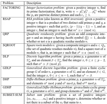
Problem Description
FACTORING Integer factorization problem: given a positive integern, find its prime factorization; that is, writen = pe1
1 pe22. . . pekk where thepiare pairwise distinct primes and eachei≥1.
RSAP RSA problem (also known as RSA inversion): given a positive integernthat is a product of two distinct odd primespandq, a positive integeresuch thatgcd(e,(p−1)(q−1)) = 1, and an integerc, find an integermsuch thatme≡c (mod n). QRP Quadratic residuosity problem: given an odd composite
inte-gernand an integerahaving Jacobi symbol an = 1, decide whether or notais a quadratic residue modulon.
SQROOT Square roots modulon: given a composite integernanda∈Qn (the set of quadratic residues modulon), find a square root ofa modulon; that is, an integerxsuch thatx2≡a (modn).
DLP Discrete logarithm problem: given a primep, a generatorαof
Z∗p, and an elementβ∈Z∗p, find the integerx,0≤x≤p−2, such thatαx≡β (modp).
GDLP Generalized discrete logarithm problem: given a finite cyclic groupGof ordern, a generatorαofG, and an elementβ ∈G, find the integerx,0≤x≤n−1, such thatαx=β.
DHP Diffie-Hellman problem: given a primep, a generatorαofZ∗p, and elementsαamodpandαbmodp, findαabmodp. GDHP Generalized Diffie-Hellman problem: given a finite cyclic group
G, a generatorαofG, and group elementsαaandαb, findαab. SUBSET-SUM Subset sum problem: given a set of positive integers
{a1, a2, . . . , an}and a positive integers, determine whether or not there is a subset of theajthat sums tos.
Table 3.1:Some computational problems of cryptographic relevance.
computational problem to another have been devised and studied in the literature. These re-ductions provide a means for converting any algorithm that solves the second problem into an algorithm for solving the first problem. The following intuitive notion of reducibility (cf.§2.3.3) is used in this chapter.
3.1 Definition LetAandBbe two computational problems.Ais said to polytime reduce to B, writtenA≤P B, if there is an algorithm that solvesAwhich uses, as a subroutine, a hypothetical algorithm for solvingB, and which runs in polynomial time if the algorithm forBdoes.3
Informally speaking, ifApolytime reduces toB, thenB is at least as difficult asA; equivalently,Ais no harder thanB. Consequently, ifAis a well-studied computational problem that is widely believed to be intractable, then proving thatA≤P Bprovides strong evidence of the intractability of problemB.
3.2 Definition LetAandBbe two computational problems. IfA≤P BandB≤P A, then AandBare said to be computationally equivalent, writtenA≡P B.
3
§3.2 The integer factorization problem 89
Informally speaking, if A≡P B thenAandB are either both tractable or both in-tractable, as the case may be.
Chapter outline
The remainder of the chapter is organized as follows. Algorithms for the integer factoriza-tion problem are studied in§3.2. Two problems related to factoring, the RSA problem and the quadratic residuosity problem, are briefly considered in§3.3 and§3.4. Efficient algo-rithms for computing square roots inZp,pa prime, are presented in§3.5, and the equiva-lence of the problems of finding square roots modulo a composite integernand factoring nis established. Algorithms for the discrete logarithm problem are studied in§3.6, and the related Diffie-Hellman problem is briefly considered in§3.7. The relation between the problems of factoring a composite integernand computing discrete logarithms in (cyclic subgroups of) the groupZ∗n is investigated in§3.8. The tasks of finding partial solutions to the discrete logarithm problem, the RSA problem, and the problem of computing square roots modulo a composite integernare the topics of§3.9. TheL3-lattice basis reduction
algorithm is presented in§3.10, along with algorithms for the subset sum problem and for simultaneous diophantine approximation. Berlekamp’sQ-matrix algorithm for factoring polynomials is presented in§3.11. Finally,§3.12 provides references and further chapter notes.
3.2 The integer factorization problem
The security of many cryptographic techniques depends upon the intractability of the in-teger factorization problem. A partial list of such protocols includes the RSA public-key encryption scheme (§8.2), the RSA signature scheme (§11.3.1), and the Rabin public-key encryption scheme (§8.3). This section summarizes the current knowledge on algorithms for the integer factorization problem.
3.3 Definition The integer factorization problem (FACTORING) is the following: given a positive integern, find its prime factorization; that is, writen=pe1
1 pe22· · ·pekk where the piare pairwise distinct primes and eachei≥1.
3.4 Remark (primality testing vs. factoring) The problem of deciding whether an integer is composite or prime seems to be, in general, much easier than the factoring problem. Hence, before attempting to factor an integer, the integer should be tested to make sure that it is indeed composite. Primality tests are a main topic of Chapter 4.
3.5 Remark (splitting vs. factoring) A non-trivial factorization ofnis a factorization of the formn=abwhere1< a < nand1< b < n;aandbare said to be non-trivial factors ofn. Hereaandbare not necessarily prime. To solve the integer factorization problem, it suffices to study algorithms that splitn, that is, find a non-trivial factorizationn=ab. Once found, the factorsaandbcan be tested for primality. The algorithm for splitting integers can then be recursively applied toaand/orb, if either is found to be composite. In this manner, the prime factorization ofncan be obtained.
p≤lgn, an integer approximationxofn1/pis computed. This can be done by performing a binary search forxsatisfyingn=xpin the interval[2,2⌊lgn/p⌋+1]. The entire procedure
takesO((lg3n) lg lg lgn)bit operations. For the remainder of this section, it will always be assumed thatnis not a perfect power. It follows that ifnis composite, thennhas at least two distinct prime factors.
Some factoring algorithms are tailored to perform better when the integernbeing fac-tored is of a special form; these are called special-purpose factoring algorithms. The run-ning times of such algorithms typically depend on certain properties of the factors ofn. Ex-amples of special-purpose factoring algorithms include trial division (§3.2.1), Pollard’s rho algorithm (§3.2.2), Pollard’sp−1algorithm (§3.2.3), the elliptic curve algorithm (§3.2.4), and the special number field sieve (§3.2.7). In contrast, the running times of the so-called general-purpose factoring algorithms depend solely on the size ofn. Examples of general-purpose factoring algorithms include the quadratic sieve (§3.2.6) and the general number field sieve (§3.2.7).
Whenever applicable, special-purpose algorithms should be employed as they will gen-erally be more efficient. A reasonable overall strategy is to attempt to find small factors first, capitalize on any particular special forms an integer may have, and then, if all else fails, bring out the general-purpose algorithms. As an example of a general strategy, one might consider the following.
1. Apply trial division by small primes less than some boundb1.
2. Next, apply Pollard’s rho algorithm, hoping to find any small prime factors smaller than some boundb2, whereb2> b1.
3. Apply the elliptic curve factoring algorithm, hoping to find any small factors smaller than some boundb3, whereb3> b2.
4. Finally, apply one of the more powerful general-purpose algorithms (quadratic sieve or general number field sieve).
3.2.1 Trial division
Once it is established that an integernis composite, before expending vast amounts of time with more powerful techniques, the first thing that should be attempted is trial division by all “small” primes. Here, “small” is determined as a function of the size ofn. As an extreme case, trial division can be attempted by all primes up to√n. If this is done, trial division will completely factornbut the procedure will take roughly√ndivisions in the worst case whennis a product of two primes of the same size. In general, if the factors found at each stage are tested for primality, then trial division to factorncompletely takesO(p+ lgn) divisions, wherepis the second-largest prime factor ofn.
Fact 3.7 indicates that if trial division is used to factor a randomly chosen large integer n, then the algorithm can be expected to find some small factors ofnrelatively quickly, and expend a large amount of time to find the second largest prime factor ofn.
3.7 Fact Letnbe chosen uniformly at random from the interval[1, x].
(i) If 12 ≤ α ≤ 1, then the probability that the largest prime factor ofnis≤ xα is approximately1 + lnα. Thus, for example, the probability thatnhas a prime factor >√xisln 2≈0.69.
(ii) The probability that the second-largest prime factor ofnis≤x0.2117is about 1 2.
(iii) The expected total number of prime factors ofnisln lnx+O(1). (Ifn=Qpei
§3.2 The integer factorization problem 91
3.2.2 Pollard’s rho factoring algorithm
Pollard’s rho algorithm is a special-purpose factoring algorithm for finding small factors of a composite integer.
Letf : S −→ Sbe a random function, whereSis a finite set of cardinalityn. Let x0be a random element ofS, and consider the sequencex0, x1, x2, . . . defined byxi+1=
f(xi)fori ≥ 0. SinceS is finite, the sequence must eventually cycle, and consists of a tail of expected lengthpπn/8followed by an endlessly repeating cycle of expected length p
πn/8(see Fact 2.37). A problem that arises in some cryptanalytic tasks, including integer factorization (Algorithm 3.9) and the discrete logarithm problem (Algorithm 3.60), is of finding distinct indicesiandjsuch thatxi=xj(a collision is then said to have occurred). An obvious method for finding a collision is to compute and storexifori= 0,1,2, . . . and look for duplicates. The expected number of inputs that must be tried before a duplicate is detected ispπn/2(Fact 2.27). This method requiresO(√n)memory andO(√n)time, assuming thexiare stored in a hash table so that new entries can be added in constant time.
3.8 Note (Floyd’s cycle-finding algorithm) The large storage requirements in the above tech-nique for finding a collision can be eliminated by using Floyd’s cycle-finding algorithm. In this method, one starts with the pair(x1, x2), and iteratively computes(xi, x2i)from the previous pair(xi−1, x2i−2), untilxm =x2mfor somem. If the tail of the sequence has lengthλand the cycle has lengthµ, then the first time thatxm =x2mis whenm = µ(1 +⌊λ/µ⌋). Note thatλ < m≤λ+µ, and consequently the expected running time of this method isO(√n).
Now, letpbe a prime factor of a composite integern. Pollard’s rho algorithm for fac-toringnattempts to find duplicates in the sequence of integersx0, x1, x2, . . . defined by
x0= 2,xi+1=f(xi) =x2i + 1 modpfori≥0. Floyd’s cycle-finding algorithm is uti-lized to findxmandx2msuch thatxm≡x2m (modp). Sincepdividesnbut is unknown, this is done by computing the termsximodulonand testing ifgcd(xm−x2m, n) > 1. If alsogcd(xm−x2m, n) < n, then a non-trivial factor ofnis obtained. (The situation gcd(xm−x2m, n) =noccurs with negligible probability.)
3.9 AlgorithmPollard’s rho algorithm for factoring integers
INPUT: a composite integernthat is not a prime power. OUTPUT: a non-trivial factordofn.
1. Seta←2,b←2.
2. Fori= 1,2, . . . do the following:
2.1 Computea←a2+ 1 modn, b←b2+ 1 modn, b←b2+ 1 modn.
2.2 Computed= gcd(a−b, n).
2.3 If1< d < nthen return(d) and terminate with success.
2.4 Ifd=nthen terminate the algorithm with failure (see Note 3.12).
a b d
5 26 1
26 2871 1
677 179685 1 2871 155260 1 44380 416250 1 179685 43670 1 121634 164403 1 155260 247944 1 44567 68343 743
Hence two non-trivial factors of455459are743and455459/743 = 613.
3.11 Fact Assuming that the functionf(x) =x2+ 1 modpbehaves like a random function,
the expected time for Pollard’s rho algorithm to find a factorpofnisO(√p)modular mul-tiplications. This implies that the expected time to find a non-trivial factor ofnisO(n1/4)
modular multiplications.
3.12 Note (options upon termination with failure) If Pollard’s rho algorithm terminates with failure, one option is to try again with a different polynomialf having integer coefficients instead off(x) = x2+ 1. For example, the polynomialf(x) =x2+cmay be used as
long asc6= 0,−2.
3.2.3 Pollard’s
p
−
1
factoring algorithm
Pollard’sp−1factoring algorithm is a special-purpose factoring algorithm that can be used to efficiently find any prime factorspof a composite integernfor whichp−1is smooth (see Definition 3.13) with respect to some relatively small boundB.
3.13 Definition LetB be a positive integer. An integernis said to beB-smooth, or smooth with respect to a boundB, if all its prime factors are≤B.
The idea behind Pollard’sp−1algorithm is the following. LetB be a smoothness bound. LetQbe the least common multiple of all powers of primes≤Bthat are≤n. If ql≤n, thenllnq≤lnn, and sol≤ ⌊lnn
lnq⌋. Thus Q = Y
q≤B
q⌊lnn/lnq⌋,
§3.2 The integer factorization problem 93
3.14 AlgorithmPollard’sp−1algorithm for factoring integers
INPUT: a composite integernthat is not a prime power. OUTPUT: a non-trivial factordofn.
1. Select a smoothness boundB.
2. Select a random integera,2≤a ≤n−1, and computed= gcd(a, n). Ifd ≥2 then return(d).
3. For each primeq≤Bdo the following: 3.1 Computel=⌊lnlnnq⌋.
3.2 Computea←aql
modn(using Algorithm 2.143). 4. Computed= gcd(a−1, n).
5. Ifd= 1ord=n, then terminate the algorithm with failure. Otherwise, return(d).
3.15 Example (Pollard’sp−1algorithm for finding a non-trivial factor ofn= 19048567) 1. Select the smoothness boundB= 19.
2. Select the integera= 3and computegcd(3, n) = 1.
3. The following table lists the intermediate values of the variablesq,l, andaafter each iteration of step 3 in Algorithm 3.14:
q l a
2 24 2293244 3 15 13555889 5 10 16937223 7 8 15214586 11 6 9685355 13 6 13271154 17 5 11406961
19 5 554506
4. Computed= gcd(554506−1, n) = 5281.
5. Two non-trivial factors ofnarep= 5281andq=n/p= 3607(these factors are in fact prime).
Notice thatp−1 = 5280 = 25×3×5×11, andq−1 = 3606 = 2×3×601. That
is,p−1is19-smooth, whileq−1is not19-smooth.
3.16 Fact Letnbe an integer having a prime factorpsuch thatp−1isB-smooth. The run-ning time of Pollard’sp−1algorithm for finding the factorpisO(Blnn/lnB)modular multiplications.
3.17 Note (improvements) The smoothness boundBin Algorithm 3.14 is selected based on the amount of time one is willing to spend on Pollard’sp−1algorithm before moving on to more general techniques. In practice,B may be between105and106. If the algorithm
terminates withd = 1, then one might try searching over prime numbersq1, q2, . . . , ql larger thanBby first computinga←aqi modnfor1 ≤i ≤ l, and then computingd =
3.2.4 Elliptic curve factoring
The details of the elliptic curve factoring algorithm are beyond the scope of this book; nev-ertheless, a rough outline follows. The success of Pollard’sp−1algorithm hinges onp−1 being smooth for some prime divisorpofn; if no suchpexists, then the algorithm fails. Observe thatp−1is the order of the groupZ∗p. The elliptic curve factoring algorithm is a generalization of Pollard’sp−1algorithm in the sense that the groupZ∗pis replaced by a random elliptic curve group overZp. The order of such a group is roughly uniformly dis-tributed in the interval[p+1−2√p, p+1+2√p]. If the order of the group chosen is smooth with respect to some pre-selected bound, the elliptic curve algorithm will, with high prob-ability, find a non-trivial factor ofn. If the group order is not smooth, then the algorithm will likely fail, but can be repeated with a different choice of elliptic curve group.
The elliptic curve algorithm has an expected running time ofLp[12,
√
2](see Exam-ple 2.61 for definition ofLp) to find a factorpofn. Since this running time depends on the size of the prime factors ofn, the algorithm tends to find small such factors first. The elliptic curve algorithm is, therefore, classified as a special-purpose factoring algorithm. It is currently the algorithm of choice for findingt-decimal digit prime factors, fort≤40, of very large composite integers.
In the hardest case, whennis a product of two primes of roughly the same size, the expected running time of the elliptic curve algorithm isLn[12,1], which is the same as that of the quadratic sieve (§3.2.6). However, the elliptic curve algorithm is not as efficient as the quadratic sieve in practice for such integers.
3.2.5 Random square factoring methods
The basic idea behind the random square family of methods is the following. Supposex andy are integers such thatx2 ≡ y2 (modn)butx 6≡ ±y (mod n). Thenndivides
x2−y2= (x−y)(x+y)butndoes not divide either(x−y)or(x+y). Hence,gcd(x−y, n)
must be a non-trivial factor ofn. This result is summarized next.
3.18 Fact Letx,y, andnbe integers. Ifx2≡y2 (modn)butx6≡ ±y (modn), thengcd(x−
y, n)is a non-trivial factor ofn.
The random square methods attempt to find integersxandy at random so thatx2 ≡ y2
(mod n). Then, as shown in Fact 3.19, with probability at least12it is the case thatx6≡ ±y (mod n), whencegcd(x−y, n)will yield a non-trivial factor ofn.
3.19 Fact Letnbe an odd composite integer that is divisible bykdistinct odd primes. Ifa ∈
Z∗n, then the congruencex2 ≡ a2 (modn)has exactly2k solutions modulon, two of which arex=aandx=−a.
3.20 Example Letn= 35. Then there are four solutions to the congruencex2≡4 (mod 35),
namelyx= 2,12,23, and33.
A common strategy employed by the random square algorithms for findingxandyat random satisfyingx2≡y2 (mod n)is the following. A set consisting of the firsttprimes
S={p1, p2, . . . , pt}is chosen;Sis called the factor base. Proceed to find pairs of integers (ai, bi)satisfying
(i) a2
§3.2 The integer factorization problem 95
(ii) bi =Qtj=1p
eij
j ,eij ≥0; that is,biispt-smooth.
Next find a subset of thebi’s whose product is a perfect square. Knowing the factoriza-tions of thebi’s, this is possible by selecting a subset of thebi’s such that the power of each primepj appearing in their product is even. For this purpose, only the parity of the non-negative integer exponentseij needs to be considered. Thus, to simplify matters, for eachi, associate the binary vectorvi= (vi1, vi2, . . . , vit)with the integer exponent vector (ei1, ei2, . . . , eit)such thatvij =eij mod 2. Ift+ 1pairs(ai, bi)are obtained, then the t-dimensional vectorsv1, v2, . . . , vt+1must be linearly dependent overZ2. That is, there
must exist a non-empty subsetT ⊆ {1,2, . . . , t+ 1}such thatPi∈Tvi= 0overZ2, and
henceQi∈Tbiis a perfect square. The setTcan be found using ordinary linear algebra over
Z2. Clearly,Qi∈Ta2i is also a perfect square. Thus settingx= Q
i∈Taiandyto be the integer square root ofQi∈Tbiyields a pair of integers(x, y)satisfyingx2≡y2 (modn). If this pair also satisfiesx6≡ ±y (modn), thengcd(x−y, n)yields a non-trivial factor ofn. Otherwise, some of the(ai, bi)pairs may be replaced by some new such pairs, and the process is repeated. In practice, there will be several dependencies among the vectors v1, v2, . . . , vt+1, and with high probability at least one will yield an(x, y)pair satisfying
x 6≡ ±y (modn); hence, this last step of generating new(ai, bi)pairs does not usually occur.
This description of the random square methods is incomplete for two reasons. Firstly, the optimal choice oft, the size of the factor base, is not specified; this is addressed in Note 3.24. Secondly, a method for efficiently generating the pairs(ai, bi)is not specified. Several techniques have been proposed. In the simplest of these, called Dixon’s algorithm, aiis chosen at random, andbi =a2i modnis computed. Next, trial division by elements in the factor base is used to test whetherbiispt-smooth. If not, then another integeraiis chosen at random, and the procedure is repeated.
The more efficient techniques strategically select anaisuch thatbiis relatively small. Since the proportion ofpt-smooth integers in the interval[2, x]becomes larger asx de-creases, the probability of suchbi beingpt-smooth is higher. The most efficient of such techniques is the quadratic sieve algorithm, which is described next.
3.2.6 Quadratic sieve factoring
Suppose an integernis to be factored. Letm=⌊√n⌋, and consider the polynomialq(x) = (x+m)2−n. Note that
q(x) = x2+ 2mx+m2−n ≈ x2+ 2mx, (3.1)
which is small (relative ton) ifxis small in absolute value. The quadratic sieve algorithm selectsai = (x+m)and tests whetherbi = (x+m)2 −nispt-smooth. Note that a2
3.21 AlgorithmQuadratic sieve algorithm for factoring integers
INPUT: a composite integernthat is not a prime power. OUTPUT: a non-trivial factordofn.
1. Select the factor baseS = {p1, p2, . . . , pt}, wherep1 =−1andpj (j ≥ 2) is the
by elements inSwhetherbispt-smooth. If not, pick a newxand repeat step 3.1. 3.2 Ifbispt-smooth, sayb =Qtj=1p
3.22 Example (quadratic sieve algorithm for finding a non-trivial factor ofn= 24961) 1. Select the factor baseS ={−1,2,3,5,13,23}of sizet = 6. (7,11,17and19are
8. Since936≡ −24025 (modn), another linear dependency must be found. 9. By inspection,v3+v6+v7= 0; thusT ={3,6,7}.
10. Computex= (a3a6a7modn) = 23405.
§3.2 The integer factorization problem 97
12. Computey= (−25·32·53modn) = 13922.
13. Now,234056≡ ±13922 (modn), so computegcd(x−y, n) = gcd(9483,24961) = 109. Hence, two non-trivial factors of24961are109and229.
3.23 Note (sieving) Instead of testing smoothness by trial division in step 3.1 of Algorithm 3.21, a more efficient technique known as sieving is employed in practice. Observe first that ifp is an odd prime in the factor base andpdividesq(x), thenpalso dividesq(x+lp)for every integerl. Thus by solving the equationq(x) ≡0 (modp)forx(for example, using the algorithms in§3.5.1), one knows either one or two (depending on the number of solutions to the quadratic equation) entire sequences of other valuesyfor whichpdividesq(y).
The sieving process is the following. An arrayQ[ ]indexed byx,−M ≤x≤M, is created and thexthentry is initialized to⌊lg|q(x)|⌋. Letx
1,x2be the solutions toq(x)≡0
(mod p), wherepis an odd prime in the factor base. Then the value⌊lgp⌋is subtracted from those entriesQ[x]in the array for whichx≡x1orx2 (mod p)and−M≤x≤M.
This is repeated for each odd primepin the factor base. (The case ofp = 2and prime powers can be handled in a similar manner.) After the sieving, the array entriesQ[x]with values near0are most likely to bept-smooth (roundoff errors must be taken into account), and this can be verified by factoringq(x)by trial division.
3.24 Note (running time of the quadratic sieve) To optimize the running time of the quadratic sieve, the size of the factor base should be judiciously chosen. The optimal selection of t ≈ Ln[12,12](see Example 2.61) is derived from knowledge concerning the distribution of smooth integers close to√n. With this choice, Algorithm 3.21 with sieving (Note 3.23) has an expected running time ofLn[12,1], independent of the size of the factors ofn.
3.25 Note (multiple polynomial variant) In order to collect a sufficient number of(ai, bi)pairs, the sieving interval must be quite large. From equation (3.1) it can be seen that|q(x)| in-creases linearly with|x|, and consequently the probability of smoothness decreases. To overcome this problem, a variant (the multiple polynomial quadratic sieve) was proposed whereby many appropriately-chosen quadratic polynomials can be used instead of justq(x), each polynomial being sieved over an interval of much smaller length. This variant also has an expected running time ofLn[12,1], and is the method of choice in practice.
3.26 Note (parallelizing the quadratic sieve) The multiple polynomial variant of the quadratic sieve is well suited for parallelization. Each node of a parallel computer, or each computer in a network of computers, simply sieves through different collections of polynomials. Any (ai, bi)pair found is reported to a central processor. Once sufficient pairs have been col-lected, the corresponding system of linear equations is solved on a single (possibly parallel) computer.
3.27 Note (quadratic sieve vs. elliptic curve factoring) The elliptic curve factoring algorithm (§3.2.4) has the same4expected (asymptotic) running time as the quadratic sieve factoring algorithm in the special case whennis the product of two primes of equal size. However, for such numbers, the quadratic sieve is superior in practice because the main steps in the algorithm are single precision operations, compared to the much more computationally in-tensive multi-precision elliptic curve operations required in the elliptic curve algorithm.
4
3.2.7 Number field sieve factoring
For several years it was believed by some people that a running time ofLn[12,1]was, in fact, the best achievable by any integer factorization algorithm. This barrier was broken in 1990 with the discovery of the number field sieve. Like the quadratic sieve, the number field sieve is an algorithm in the random square family of methods (§3.2.5). That is, it attempts to find integersxandysuch thatx2≡y2 (modn)andx6≡ ±y (mod n). To achieve this
goal, two factor bases are used, one consisting of all prime numbers less than some bound, and the other consisting of all prime ideals of norm less than some bound in the ring of integers of a suitably-chosen algebraic number field. The details of the algorithm are quite complicated, and are beyond the scope of this book.
A special version of the algorithm (the special number field sieve) applies to integers of the formn=re−sfor smallrand|s|, and has an expected running time ofL
n[13, c], wherec= (32/9)1/3≈1.526.
The general version of the algorithm, sometimes called the general number field sieve, applies to all integers and has an expected running time ofLn[13, c], wherec= (64/9)1/3≈ 1.923. This is, asymptotically, the fastest algorithm known for integer factorization. The primary reason why the running time of the number field sieve is smaller than that of the quadratic sieve is that the candidate smooth numbers in the former are much smaller than those in the latter.
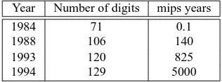
The general number field sieve was at first believed to be slower than the quadratic sieve for factoring integers having fewer than 150 decimal digits. However, experiments in 1994–1996 have indicated that the general number field sieve is substantially faster than the quadratic sieve even for numbers in the 115 digit range. This implies that the crossover point between the effectiveness of the quadratic sieve vs. the general number field sieve may be 110–120 digits. For this reason, the general number field sieve is considered the current champion of all general-purpose factoring algorithms.
3.3 The RSA problem
The intractability of the RSA problem forms the basis for the security of the RSA public-key encryption scheme (§8.2) and the RSA signature scheme (§11.3.1).
3.28 Definition The RSA problem (RSAP) is the following: given a positive integernthat is a product of two distinct odd primespandq, a positive integeresuch thatgcd(e,(p−1)(q−
1)) = 1, and an integerc, find an integermsuch thatme≡c (modn).
In other words, the RSA problem is that of findingethroots modulo a composite integer
n. The conditions imposed on the problem parametersnandeensure that for each integer c ∈ {0,1, . . . , n −1}there is exactly onem ∈ {0,1, . . . , n−1}such thatme ≡ c (mod n). Equivalently, the functionf :Zn −→Zndefined asf(m) =memodnis a permutation.
§3.4 The quadratic residuosity problem 99
As is shown in§8.2.2(i), if the factors ofnare known then the RSA problem can be easily solved. This fact is stated next.
3.30 Fact RSAP≤P FACTORING. That is, the RSA problem polytime reduces to the integer factorization problem.
It is widely believed that the RSA and the integer factorization problems are computa-tionally equivalent, although no proof of this is known.
3.4 The quadratic residuosity problem
The security of the Goldwasser-Micali probabilistic public-key encryption scheme (§8.7) and the Blum-Blum-Shub pseudorandom bit generator (§5.5.2) are both based on the ap-parent intractability of the quadratic residuosity problem.
Recall from§2.4.5 that ifn ≥ 3is an odd integer, then Jnis the set of alla ∈ Z∗n having Jacobi symbol 1. Recall also thatQnis the set of quadratic residues modulonand that the set of pseudosquares modulonis defined byQen=Jn−Qn.
3.31 Definition The quadratic residuosity problem (QRP) is the following: given an odd com-posite integernanda∈Jn, decide whether or notais a quadratic residue modulon.
3.32 Remark (QRP with a prime modulus) Ifnis a prime, then it is easy to decide whether a∈Z∗nis a quadratic residue modulonsince, by definition,a∈Qnif and only if na= 1, and the Legendre symbol ancan be efficiently calculated by Algorithm 2.149.
Assume now thatnis a product of two distinct odd primespandq. It follows from Fact 2.137 that ifa∈Jn, thena∈Qnif and only if ap= 1. Thus, if the factorization of nis known, then QRP can be solved simply by computing the Legendre symbol ap. This observation can be generalized to all integersnand leads to the following fact.
3.33 Fact QRP≤P FACTORING. That is, the QRP polytime reduces to the FACTORING problem.
On the other hand, if the factorization ofnis unknown, then there is no efficient pro-cedure known for solving QRP, other than by guessing the answer. Ifn = pq, then the probability of a correct guess is 12 since|Qn| =|Qen|(Fact 2.155). It is believed that the QRP is as difficult as the problem of factoring integers, although no proof of this is known.
3.5 Computing square roots in
Z
n3.5.1 Case (i):
n
prime
Recall from Remark 3.32 that ifpis a prime, then it is easy to decide ifa∈Z∗pis a quadratic residue modulop. Ifais, in fact, a quadratic residue modulop, then the two square roots ofacan be efficiently computed, as demonstrated by Algorithm 3.34.
3.34 AlgorithmFinding square roots modulo a primep
INPUT: an odd primepand an integera,1≤a≤p−1.
OUTPUT: the two square roots ofamodulop, providedais a quadratic residue modulop. 1. Compute the Legendre symbol apusing Algorithm 2.149. If ap=−1then return(a
does not have a square root modulop) and terminate.
2. Select integersb,1≤b≤p−1, at random until one is found with b p
=−1. (bis a quadratic non-residue modulop.)
3. By repeated division by2, writep−1 = 2st, wheretis odd.
4. Computea−1modpby the extended Euclidean algorithm (Algorithm 2.142).
5. Setc←btmodpandr←a(t+1)/2modp(Algorithm 2.143).
6. Forifrom 1 tos−1do the following: 6.1 Computed= (r2·a−1)2s−i−1modp.
6.2 Ifd≡ −1 (modp)then setr←r·cmodp. 6.3 Setc←c2modp.
7. Return(r,−r).
Algorithm 3.34 is a randomized algorithm because of the manner in which the quadratic non-residuebis selected in step 2. No deterministic polynomial-time algorithm for finding a quadratic non-residue modulo a primepis known (see Remark 2.151).
3.35 Fact Algorithm 3.34 has an expected running time ofO((lgp)4)bit operations.
This running time is obtained by observing that the dominant step (step 6) is executed s−1times, each iteration involving a modular exponentiation and thus takingO((lgp)3)bit
operations (Table 2.5). Since in the worst cases=O(lgp), the running time ofO((lgp)4)
follows. Whensis small, the loop in step 6 is executed only a small number of times, and the running time of Algorithm 3.34 isO((lgp)3)bit operations. This point is demonstrated
next for the special casess= 1ands= 2.
Specializing Algorithm 3.34 to the cases= 1yields the following simple deterministic algorithm for finding square roots whenp≡3 (mod 4).
3.36 AlgorithmFinding square roots modulo a primepwherep≡3 (mod 4) INPUT: an odd primepwherep≡3 (mod 4), and a squarea∈Qp. OUTPUT: the two square roots ofamodulop.
1. Computer=a(p+1)/4modp(Algorithm 2.143).
2. Return(r,−r).
§3.5 Computing square roots inZn 101
3.37 AlgorithmFinding square roots modulo a primepwherep≡5 (mod 8) INPUT: an odd primepwherep≡5 (mod 8), and a squarea∈Qp. OUTPUT: the two square roots ofamodulop.
1. Computed=a(p−1)/4modp(Algorithm 2.143).
2. Ifd= 1then computer=a(p+3)/8modp.
3. Ifd=p−1then computer= 2a(4a)(p−5)/8modp.
4. Return(r,−r).
3.38 Fact Algorithms 3.36 and 3.37 have running times ofO((lgp)3)bit operations.
Algorithm 3.39 for finding square roots modulopis preferable to Algorithm 3.34 when p−1 = 2stwithslarge.
3.39 AlgorithmFinding square roots modulo a primep
INPUT: an odd primepand a squarea∈Qp. OUTPUT: the two square roots ofamodulop.
1. Choose randomb ∈ Zp untilb2 −4ais a quadratic non-residue modulop, i.e., b2−4a
p
=−1.
2. Letfbe the polynomialx2−bx+ainZ
p[x].
3. Computer=x(p+1)/2modf using Algorithm 2.227. (Note:rwill be an integer.)
4. Return(r,−r).
3.40 Fact Algorithm 3.39 has an expected running time ofO((lgp)3)bit operations.
3.41 Note (computing square roots in a finite field) Algorithms 3.34, 3.36, 3.37, and 3.39 can be extended in a straightforward manner to find square roots in any finite fieldFqof odd order q=pm,pprime,m≥1. Square roots in finite fields of even order can also be computed efficiently via Fact 3.42.
3.42 Fact Each elementa∈F2m has exactly one square root, namelya2 m−1
.
3.5.2 Case (ii):
n
composite
The discussion in this subsection is restricted to the case of computing square roots modulo n, wherenis a product of two distinct odd primespandq. However, all facts presented here generalize to the case wherenis an arbitrary composite integer.
Unlike the case wherenis a prime, the problem of deciding whether a givena∈Z∗n is a quadratic residue modulo a composite integern, is believed to be a difficult problem. Certainly, if the Jacobi symbol na=−1, thenais a quadratic non-residue. On the other hand, if an = 1, then deciding whether or notais a quadratic residue is precisely the quadratic residuosity problem, considered in§3.4.
If the factorspandqofnare known, then the SQROOT problem can be solved effi-ciently by first finding square roots ofamodulopand moduloq, and then combining them using the Chinese remainder theorem (Fact 2.120) to obtain the square roots ofamodulo n. The steps are summarized in Algorithm 3.44, which, in fact, finds all of the four square roots ofamodulon.
3.44 AlgorithmFinding square roots modulongiven its prime factorspandq
INPUT: an integern, its prime factorspandq, anda∈Qn. OUTPUT: the four square roots ofamodulon.
1. Use Algorithm 3.39 (or Algorithm 3.36 or 3.37, if applicable) to find the two square rootsrand−rofamodulop.
2. Use Algorithm 3.39 (or Algorithm 3.36 or 3.37, if applicable) to find the two square rootssand−sofamoduloq.
3. Use the extended Euclidean algorithm (Algorithm 2.107) to find integerscanddsuch thatcp+dq= 1.
4. Setx←(rdq+scp) modnandy←(rdq−scp) modn. 5. Return(±xmodn,±ymodn).
3.45 Fact Algorithm 3.44 has an expected running time ofO((lgp)3)bit operations.
Algorithm 3.44 shows that if one can factorn, then the SQROOT problem is easy. More precisely, SQROOT≤P FACTORING. The converse of this statement is also true, as stated in Fact 3.46.
3.46 Fact FACTORING≤P SQROOT. That is, the FACTORING problem polytime reduces to the SQROOT problem. Hence, since SQROOT≤P FACTORING, the FACTORING and SQROOT problems are computationally equivalent.
Justification. Suppose that one has a polynomial-time algorithmAfor solving the SQ-ROOT problem. This algorithm can then be used to factor a given composite integernas follows. Select an integerxat random withgcd(x, n) = 1, and computea=x2modn.
Next, algorithmAis run with inputsaandn, and a square rootyofamodulonis returned. Ify ≡ ±x (mod n), then the trial fails, and the above procedure is repeated with a new xchosen at random. Otherwise, ify6≡ ±x (mod n), thengcd(x−y, n)is guaranteed to be a non-trivial factor ofn(Fact 3.18), namely,porq. Sinceahas four square roots mod-ulon(±xand±zwith±z 6≡ ±x (mod n)), the probability of success for each attempt is12. Hence, the expected number of attempts before a factor ofnis obtained is two, and
consequently the procedure runs in expected polynomial time.
3.47 Note (strengthening of Fact 3.46) The proof of Fact 3.46 can be easily modified to estab-lish the following stronger result. Letc ≥ 1be any constant. If there is an algorithmA which, givenn, can find a square root modulonin polynomial time for a(lg1n)c fraction
of all quadratic residuesa∈Qn, then the algorithmAcan be used to factornin expected polynomial time. The implication of this statement is that if the problem of factoringnis difficult, then for almost alla∈Qnit is difficult to find square roots modulon.
§3.6 The discrete logarithm problem 103
3.6 The discrete logarithm problem
The security of many cryptographic techniques depends on the intractability of the discrete logarithm problem. A partial list of these includes Diffie-Hellman key agreement and its derivatives (§12.6), ElGamal encryption (§8.4), and the ElGamal signature scheme and its variants (§11.5). This section summarizes the current knowledge regarding algorithms for solving the discrete logarithm problem.
Unless otherwise specified, algorithms in this section are described in the general set-ting of a (multiplicatively written) finite cyclic groupGof ordernwith generatorα(see Definition 2.167). For a more concrete approach, the reader may find it convenient to think ofGas the multiplicative groupZ∗pof orderp−1, where the group operation is simply multiplication modulop.
3.48 Definition LetGbe a finite cyclic group of ordern. Letαbe a generator ofG, and let β∈G. The discrete logarithm ofβto the baseα, denotedlogαβ, is the unique integerx, 0≤x≤n−1, such thatβ=αx.
3.49 Example Letp= 97. ThenZ∗97is a cyclic group of ordern= 96. A generator ofZ∗97is
α= 5. Since532≡35 (mod 97),log
535 = 32inZ∗97.
The following are some elementary facts about logarithms.
3.50 Fact Letαbe a generator of a cyclic groupGof ordern, and letβ,γ ∈G. Letsbe an integer. Thenlogα(βγ) = (logαβ+ logαγ) modnandlogα(βs) =slog
αβmodn. The groups of most interest in cryptography are the multiplicative groupF∗qof the finite fieldFq(§2.6), including the particular cases of the multiplicative groupZ∗pof the integers modulo a primep, and the multiplicative groupF∗2mof the finite fieldF2mof characteristic
two. Also of interest are the group of unitsZ∗nwherenis a composite integer, the group of points on an elliptic curve defined over a finite field, and the jacobian of a hyperelliptic curve defined over a finite field.
3.51 Definition The discrete logarithm problem (DLP) is the following: given a primep, a generatorαofZ∗p, and an elementβ ∈ Zp∗, find the integerx,0≤x ≤p−2, such that αx≡β (modp).
3.52 Definition The generalized discrete logarithm problem (GDLP) is the following: given a finite cyclic groupGof ordern, a generatorαofG, and an elementβ∈G, find the integer x,0≤x≤n−1, such thatαx=β.
The discrete logarithm problem in elliptic curve groups and in the jacobians of hyper-elliptic curves are not explicitly considered in this section. The discrete logarithm problem inZ∗nis discussed further in§3.8.
3.53 Note (difficulty of the GDLP is independent of generator) Letαandγbe two generators of a cyclic groupGof ordern, and letβ∈G. Letx= logαβ,y= logγβ, andz= logαγ. Thenαx=β=γy= (αz)y. Consequentlyx=zymodn, and
logγβ= (logαβ) (logαγ)−1modn.
3.54 Note (generalization of GDLP) A more general formulation of the GDLP is the following: given a finite groupGand elementsα,β ∈G, find an integerxsuch thatαx=β, provided that such an integer exists. In this formulation, it is not required thatGbe a cyclic group, and, even if it is, it is not required thatαbe a generator ofG. This problem may be harder to solve, in general, than GDLP. However, in the case whereGis a cyclic group (for example ifGis the multiplicative group of a finite field) and the order ofαis known, it can be easily recognized whether an integerxsatisfyingαx=βexists. This is because of the following fact: ifGis a cyclic group,αis an element of orderninG, andβ ∈G, then there exists an integerxsuch thatαx=βif and only ifβn= 1.
3.55 Note (solving the DLP in a cyclic groupGof ordernis in essence computing an isomor-phism betweenGandZn) Even though any two cyclic groups of the same order are iso-morphic (that is, they have the same structure although the elements may be written in dif-ferent representations), an efficient algorithm for computing logarithms in one group does not necessarily imply an efficient algorithm for the other group. To see this, consider that every cyclic group of ordernis isomorphic to the additive cyclic groupZn, i.e., the set of integers{0,1,2, . . . , n−1}where the group operation is addition modulon. Moreover, the discrete logarithm problem in the latter group, namely, the problem of finding an inte-gerxsuch thatax≡b (mod n)givena, b∈Zn, is easy as shown in the following. First note that there does not exist a solutionxifd= gcd(a, n)does not divideb(Fact 2.119). Otherwise, ifddividesb, the extended Euclidean algorithm (Algorithm 2.107) can be used to find integerssandtsuch thatas+nt=d. Multiplying both sides of this equation by the integerb/dgivesa(sb/d) +n(tb/d) = b. Reducing this equation modulonyields a(sb/d)≡b (modn)and hencex= (sb/d) modnis the desired (and easily obtainable) solution.
The known algorithms for the DLP can be categorized as follows:
1. algorithms which work in arbitrary groups, e.g., exhaustive search (§3.6.1), the baby-step giant-baby-step algorithm (§3.6.2), Pollard’s rho algorithm (§3.6.3);
2. algorithms which work in arbitrary groups but are especially efficient if the order of the group has only small prime factors, e.g., Pohlig-Hellman algorithm (§3.6.4); and 3. the index-calculus algorithms (§3.6.5) which are efficient only in certain groups.
3.6.1 Exhaustive search
The most obvious algorithm for GDLP (Definition 3.52) is to successively computeα0,α1,
α2, . . . untilβ is obtained. This method takesO(n)multiplications, wherenis the order
ofα, and is therefore inefficient ifnis large (i.e. in cases of cryptographic interest).
3.6.2 Baby-step giant-step algorithm
§3.6 The discrete logarithm problem 105
3.56 AlgorithmBaby-step giant-step algorithm for computing discrete logarithms
INPUT: a generatorαof a cyclic groupGof ordern, and an elementβ∈G. OUTPUT: the discrete logarithmx= logαβ.
1. Setm←⌈√n⌉.
2. Construct a table with entries(j, αj)for0 ≤ j < m. Sort this table by second component. (Alternatively, use conventional hashing on the second component to store the entries in a hash table; placing an entry, and searching for an entry in the table takes constant time.)
3. Computeα−mand setγ←β.
4. Forifrom 0 tom−1do the following:
4.1 Check ifγis the second component of some entry in the table. 4.2 Ifγ=αj then return(x=im+j).
4.3 Setγ←γ·α−m.
Algorithm 3.56 requires storage forO(√n)group elements. The table takesO(√n) multiplications to construct, andO(√nlgn)comparisons to sort. Having constructed this table, step 4 takesO(√n)multiplications andO(√n)table look-ups. Under the assump-tion that a group multiplicaassump-tion takes more time thanlgncomparisons, the running time of Algorithm 3.56 can be stated more concisely as follows.
3.57 Fact The running time of the baby-step giant-step algorithm (Algorithm 3.56) isO(√n) group multiplications.
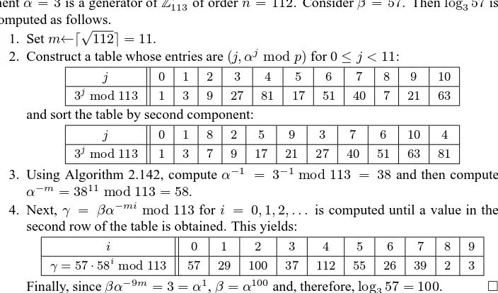
3.58 Example (baby-step giant-step algorithm for logarithms inZ∗113) Letp= 113. The
ele-mentα= 3is a generator ofZ∗113of ordern = 112. Considerβ = 57. Thenlog357is
computed as follows. 1. Setm←⌈√112⌉= 11.
2. Construct a table whose entries are(j, αjmodp)for0≤j <11:
j 0 1 2 3 4 5 6 7 8 9 10
3j
mod 113 1 3 9 27 81 17 51 40 7 21 63
and sort the table by second component:
j 0 1 8 2 5 9 3 7 6 10 4
3jmod 113 1 3 7 9 17 21 27 40 51 63 81
3. Using Algorithm 2.142, computeα−1 = 3−1mod 113 = 38and then compute
α−m= 3811mod 113 = 58.
4. Next, γ = βα−mimod 113fori = 0,1,2, . . . is computed until a value in the second row of the table is obtained. This yields:
i 0 1 2 3 4 5 6 7 8 9
γ= 57·58i
mod 113 57 29 100 37 112 55 26 39 2 3
Finally, sinceβα−9m= 3 =α1,β=α100and, therefore,log
357 = 100.
3.6.3 Pollard’s rho algorithm for logarithms
Pollard’s rho algorithm (Algorithm 3.60) for computing discrete logarithms is a randomized algorithm with the same expected running time as the baby-step giant-step algorithm (Al-gorithm 3.56), but which requires a negligible amount of storage. For this reason, it is far preferable to Algorithm 3.56 for problems of practical interest. For simplicity, it is assumed in this subsection thatGis a cyclic group whose ordernis prime.
The groupGis partitioned into three setsS1,S2, andS3of roughly equal size based
on some easily testable property. Some care must be exercised in selecting the partition; for example,16∈S2. Define a sequence of group elementsx0, x1, x2, . . . byx0= 1and
fori ≥ 0. This sequence of group elements in turn defines two sequences of integers a0, a1, a2, . . . andb0, b1, b2, . . . satisfyingxi=αaiβbifori≥0:a0= 0,b0= 0, and for
Floyd’s cycle-finding algorithm (Note 3.8) can then be utilized to find two group elements xi andx2isuch thatxi = x2i. Henceαaiβbi = αa2iβb2i, and soβbi−b2i = αa2i−ai. Taking logarithms to the baseαof both sides of this last equation yields
(bi−b2i)·logαβ ≡(a2i−ai) (mod n).
Providedbi6≡b2i (mod n)(note:bi≡b2ioccurs with negligible probability), this equa-tion can then be efficiently solved to determinelogαβ.
3.60 AlgorithmPollard’s rho algorithm for computing discrete logarithms
INPUT: a generatorαof a cyclic groupGof prime ordern, and an elementβ ∈G. OUTPUT: the discrete logarithmx= logαβ.
1. Setx0←1,a0←0,b0←0.
Ifr = 0then terminate the algorithm with failure; otherwise, compute x=r−1(a2i−ai) modnand return(x).
In the rare case that Algorithm 3.60 terminates with failure, the procedure can be re-peated by selecting random integersa0,b0in the interval[1, n−1], and starting withx0=
§3.6 The discrete logarithm problem 107
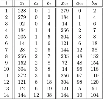
3.61 Example (Pollard’s rho algorithm for logarithms in a subgroup ofZ∗383) The elementα=
2is a generator of the subgroupGofZ∗383of ordern= 191. Supposeβ= 228. Partition
Table 3.2:Intermediate steps of Pollard’s rho algorithm in Example 3.61.
3.62 Fact LetGbe a group of ordern, a prime. Assume that the functionf : G −→ G de-fined by equation (3.2) behaves like a random function. Then the expected running time of Pollard’s rho algorithm for discrete logarithms inGisO(√n)group operations. Moreover, the algorithm requires negligible storage.
3.6.4 Pohlig-Hellman algorithm
Algorithm 3.63 for computing logarithms takes advantage of the factorization of the ordern of the groupG. Letn=pe1
1 pe22· · ·prerbe the prime factorization ofn. Ifx= logαβ, then the approach is to determinexi=xmodpieifor1≤i≤r, and then use Gauss’s algorithm (Algorithm 2.121) to recoverxmodn. Each integerxi is determined by computing the digitsl0,l1, . . . , lei−1in turn of itspi-ary representation:xi=l0+l1pi+· · ·+lei−1p
ei−1
i , where0≤lj≤pi−1.
3.63 AlgorithmPohlig-Hellman algorithm for computing discrete logarithms
INPUT: a generatorαof a cyclic groupGof ordern, and an elementβ∈G. OUTPUT: the discrete logarithmx= logαβ.
1. Find the prime factorization ofn:n=pe1
1 pe
2
2 · · ·perr, whereei≥1. 2. Forifrom 1 tordo the following:
(Computexi=l0+l1pi+· · ·+lei−1p
ei−1
i , wherexi=xmodpeii) 2.1 (Simplify the notation) Setq←piande←ei.
2.2 Setγ←1andl−1←0.
2.3 Computeα←αn/q.
2.4 (Compute thelj) Forjfrom0toe−1do the following: Computeγ←γαlj−1q
j−1
andβ←(βγ−1)n/qj+1
.
Computelj←logαβ(e.g., using Algorithm 3.56; see Note 3.67(iii)). 2.5 Setxi←l0+l1q+· · ·+le−1qe−1.
3. Use Gauss’s algorithm (Algorithm 2.121) to compute the integerx,0≤x≤n−1, such thatx≡xi (modpiei)for1≤i≤r.
4. Return(x).
Example 3.64 illustrates Algorithm 3.63 with artificially small parameters.
3.64 Example (Pohlig-Hellman algorithm for logarithms inZ∗251) Letp= 251. The element
α= 71is a generator ofZ∗251of ordern= 250. Considerβ = 210. Thenx= log71210
is computed as follows.
1. The prime factorization ofnis250 = 2·53.
2. (a) (Computex1=xmod 2)
Computeα=αn/2modp= 250andβ =βn/2modp= 250. Thenx 1 =
log250250 = 1.
(b) (Computex2=xmod 53=l0+l15 +l252)
i. Computeα=αn/5modp= 20.
ii. Computeγ = 1andβ = (βγ−1)n/5modp = 149. Using exhaustive
search,5computel0= log20149 = 2.
iii. Computeγ = γα2modp = 21andβ = (βγ−1)n/25modp = 113.
Using exhaustive search, computel1= log20113 = 4.
iv. Computeγ =γα4·5modp= 115andβ = (βγ−1)(p−1)/125modp=
149. Using exhaustive search, computel2= log20149 = 2.
Hence,x2= 2 + 4·5 + 2·52= 72.
3. Finally, solve the pair of congruencesx ≡ 1 (mod 2),x ≡ 72 (mod 125)to get
x= log71210 = 197.
3.65 Fact Given the factorization ofn, the running time of the Pohlig-Hellman algorithm (Al-gorithm 3.63) isO(Pri=1ei(lgn+√pi))group multiplications.
3.66 Note (effectiveness of Pohlig-Hellman) Fact 3.65 implies that the Pohlig-Hellman algo-rithm is efficient only if each prime divisorpiofnis relatively small; that is, ifnis a smooth
5
§3.6 The discrete logarithm problem 109
integer (Definition 3.13). An example of a group in which the Pohlig-Hellman algorithm is effective follows. Consider the multiplicative groupZ∗pwherepis the 107-digit prime:
p= 227088231986781039743145181950291021585250524967592855 96453269189798311427475159776411276642277139650833937.
The order ofZ∗pisn=p−1 = 24·1047298·2247378·3503774. Since the largest prime divisor ofp−1is only350377, it is relatively easy to compute logarithms in this group using the Pohlig-Hellman algorithm.
3.67 Note (miscellaneous)
(i) Ifnis a prime, then Algorithm 3.63 (Pohlig-Hellman) is the same as baby-step giant-step (Algorithm 3.56).
(ii) In step 1 of Algorithm 3.63, a factoring algorithm which finds small factors first (e.g., Algorithm 3.9) should be employed; if the ordernis not a smooth integer, then Al-gorithm 3.63 is inefficient anyway.
(iii) The storage required for Algorithm 3.56 in step 2.4 can be eliminated by using instead Pollard’s rho algorithm (Algorithm 3.60).
3.6.5 Index-calculus algorithm
The index-calculus algorithm is the most powerful method known for computing discrete logarithms. The technique employed does not apply to all groups, but when it does, it of-ten gives a subexponential-time algorithm. The algorithm is first described in the general setting of a cyclic groupG(Algorithm 3.68). Two examples are then presented to illustrate how the index-calculus algorithm works in two kinds of groups that are used in practical applications, namelyZ∗p(Example 3.69) andF∗2m(Example 3.70).
The index-calculus algorithm requires the selection of a relatively small subsetS of elements ofG, called the factor base, in such a way that a significant fraction of elements ofGcan be efficiently expressed as products of elements fromS. Algorithm 3.68 proceeds to precompute a database containing the logarithms of all the elements inS, and then reuses this database each time the logarithm of a particular group element is required.
The description of Algorithm 3.68 is incomplete for two reasons. Firstly, a technique for selecting the factor baseSis not specified. Secondly, a method for efficiently generating relations of the form (3.5) and (3.7) is not specified. The factor baseSmust be a subset of Gthat is small (so that the system of equations to be solved in step 3 is not too large), but not too small (so that the expected number of trials to generate a relation (3.5) or (3.7) is not too large). Suitable factor bases and techniques for generating relations are known for some cyclic groups includingZ∗p(see§3.6.5(i)) andF∗2m(see§3.6.5(ii)), and, moreover, the
multiplicative groupF∗qof a general finite fieldFq.
3.68 AlgorithmIndex-calculus algorithm for discrete logarithms in cyclic groups
INPUT: a generatorαof a cyclic groupGof ordern, and an elementβ∈G. OUTPUT: the discrete logarithmy= logαβ.
1. (Select a factor baseS) Choose a subsetS={p1, p2, . . . , pt}ofGsuch that a “sig-nificant proportion” of all elements inGcan be efficiently expressed as a product of elements fromS.
2.1 Select a random integerk,0≤k≤n−1, and computeαk. 2.2 Try to writeαkas a product of elements inS:
αk= t Y
i=1
pci
i , ci≥0. (3.5)
If successful, take logarithms of both sides of equation (3.5) to obtain a linear relation
k≡
t X
i=1
cilogαpi (mod n). (3.6)
2.3 Repeat steps 2.1 and 2.2 untilt+crelations of the form (3.6) are obtained (c is a small positive integer, e.g.c= 10, such that the system of equations given by thet+crelations has a unique solution with high probability).
3. (Find the logarithms of elements inS) Working modulon, solve the linear system oft+cequations (intunknowns) of the form (3.6) collected in step 2 to obtain the values oflogαpi,1≤i≤t.
4. (Computey)
4.1 Select a random integerk,0≤k≤n−1, and computeβ·αk. 4.2 Try to writeβ·αkas a product of elements inS:
β·αk= t Y
i=1
pdi
i , di≥0. (3.7)
If the attempt is unsuccessful then repeat step 4.1. Otherwise, taking logarithms of both sides of equation (3.7) yieldslogαβ= (Pti=1dilogαpi−k) modn; thus, computey= (Pti=1dilogαpi−k) modnand return(y).
(i) Index-calculus algorithm inZ∗p
For the fieldZp,pa prime, the factor baseScan be chosen as the firsttprime numbers. A relation (3.5) is generated by computingαkmodpand then using trial division to check whether this integer is a product of primes inS. Example 3.69 illustrates Algorithm 3.68 inZ∗pon a problem with artificially small parameters.
3.69 Example (Algorithm 3.68 for logarithms inZ∗229) Letp = 229. The elementα = 6is
a generator ofZ∗229of ordern = 228. Considerβ = 13. Thenlog613is computed as
follows, using the index-calculus technique.
1. The factor base is chosen to be the first5primes:S={2,3,5,7,11}.
2. The following six relations involving elements of the factor base are obtained (un-successful attempts are not shown):
6100mod 229 = 180 = 22·32·5 618mod 229 = 176 = 24·11 612mod 229 = 165 = 3·5·11 662mod 229 = 154 = 2·7·11
§3.6 The discrete logarithm problem 111
These relations yield the following six equations involving the logarithms of ele-ments in the factor base:
100 ≡ 2 log62 + 2 log63 + log65 (mod 228) 18 ≡ 4 log62 + log611 (mod 228)
12 ≡ log63 + log65 + log611 (mod 228) 62 ≡ log62 + log67 + log611 (mod 228) 143 ≡ log62 + 2 log63 + log611 (mod 228) 206 ≡ log62 + log63 + log65 + log67 (mod 228).
3. Solving the linear system of six equations in five unknowns (the logarithmsxi = log6pi) yields the solutionslog62 = 21,log63 = 208,log65 = 98,log67 = 107,
andlog611 = 162.
4. Suppose that the integerk = 77is selected. Sinceβ·αk = 13·677mod 229 =
147 = 3·72, it follows that
log613 = (log63 + 2 log67−77) mod 228 = 117.
(ii) Index-calculus algorithm inF∗2m
The elements of the finite fieldF2m are represented as polynomials inZ2[x]of degree at
mostm−1, where multiplication is performed modulo a fixed irreducible polynomialf(x) of degreeminZ2[x](see§2.6). The factor baseScan be chosen as the set of all irreducible
polynomials inZ2[x]of degree at most some prescribed boundb. A relation (3.5) is
gener-ated by computingαkmodf(x)and then using trial division to check whether this poly-nomial is a product of polypoly-nomials inS. Example 3.70 illustrates Algorithm 3.68 inF∗2m
on a problem with artificially small parameters.
3.70 Example (Algorithm 3.68 for logarithms inF∗27) The polynomialf(x) =x7+x+ 1is
irreducible overZ2. Hence, the elements of the finite fieldF27 of order128can be
repre-sented as the set of all polynomials inZ2[x]of degree at most6, where multiplication is
performed modulof(x). The order ofF∗27 isn= 27−1 = 127, andα=xis a generator
ofF∗27. Supposeβ=x4+x3+x2+x+ 1. Theny= logxβcan be computed as follows,
using the index-calculus technique.
1. The factor base is chosen to be the set of all irreducible polynomials inZ2[x]of degree
at most3:S={x, x+ 1, x2+x+ 1, x3+x+ 1, x3+x2+ 1}.
2. The following five relations involving elements of the factor base are obtained (un-successful attempts are not shown):
x18modf(x) =x6+x4 =x4(x+ 1)2
x105modf(x) =x6+x5+x4+x =x(x+ 1)2(x3+x2+ 1) x72modf(x) =x6+x5+x3+x2 =x2(x+ 1)2(x2+x+ 1)
x45modf(x) =x5+x2+x+ 1 = (x+ 1)2(x3+x+ 1) x121modf(x) =x6+x5+x4+x3+x2+x+ 1 = (x3+x+ 1)(x3+x2+1).
1),p3= logx(x2+x+ 1),p4= logx(x3+x+ 1), andp5= logx(x3+x2+ 1)): 18 ≡ 4p1+ 2p2 (mod 127)
105 ≡ p1+ 2p2+p5 (mod 127)
72 ≡ 2p1+ 2p2+p3 (mod 127)
45 ≡ 2p2+p4 (mod 127)
121 ≡ p4+p5 (mod 127).
3. Solving the linear system of five equations in five unknowns yields the valuesp1= 1,
p2= 7,p3= 56,p4= 31, andp5= 90.
4. Supposek= 66is selected. Since
βαk = (x4+x3+x2+x+ 1)x66modf(x) =x5+x3+x=x(x2+x+ 1)2,
it follows that
logx(x4+x3+x2+x+ 1) = (p1+ 2p3−66) mod 127 = 47.
3.71 Note (running time of Algorithm 3.68) To optimize the running time of the index-calculus algorithm, the sizetof the factor base should be judiciously chosen. The optimal selection relies on knowledge concerning the distribution of smooth integers in the interval[1, p−1] for the case ofZ∗p, and for the case ofF∗2m on the distribution of smooth polynomials (that
is, polynomials all of whose irreducible factors have relatively small degrees) among poly-nomials inF2[x]of degree less thanm. With an optimal choice oft, the index-calculus
al-gorithm as described above forZ∗pandF∗2mhas an expected running time ofLq[12, c]where
q=porq= 2m, andc >0is a constant.
3.72 Note (fastest algorithms known for discrete logarithms inZ∗pandF∗2m) Currently, the best
algorithm known for computing logarithms inF∗2mis a variation of the index-calculus
algo-rithm called Coppersmith’s algoalgo-rithm, with an expected running time ofL2m[1
3, c]for some
constantc <1.587. The best algorithm known for computing logarithms inZ∗pis a varia-tion of the index-calculus algorithm called the number field sieve, with an expected running time ofLp[13,1.923]. The latest efforts in these directions are surveyed in the Notes section (§3.12).
3.73 Note (parallelization of the index-calculus algorithm)
(i) For the optimal choice of parameters, the most time-consuming phase of the index-calculus algorithm is usually the generation of relations involving factor base loga-rithms (step 2 of Algorithm 3.68). The work for this stage can be easily distributed among a network of processors by simply having the processors search for relations independently of each other. The relations generated are collected by a central pro-cessor. When enough relations have been generated, the corresponding system of lin-ear equations can be solved (step 3 of Algorithm 3.68) on a single (possibly parallel) computer.