Estimating Driving Behavior by a Smartphone
* 1,2H.Eren,
1,2S.Makinist,
1,2E.Akin, and
3A.Yilmaz
1Firat University,
2iDaSuCo Research Inc., Elazig, Turkey3
PCVLab., The Ohio State University, Columbus, OH
Abstract—In this paper, we propose an approach to
understand the driver behavior using smartphone sensors. The aim for analyzing the sensory data acquired using a smartphone is to design a car-independent system which does not need vehicle mounted sensors measuring turn rates, gas consumption or tire pressure. The sensory data utilized in this paper includes the accelerometer, gyroscope and the magnetometer. Using these sensors we obtain position, speed, acceleration, deceleration and deflection angle sensory information and estimate commuting safety by statistically analyzing driver behavior. In contrast to state of the art, this work uses no external sensors, resulting in a cost efficient, simplistic and user-friendly system.
Key words: Driver behavior, accelerometer, gyroscope,
magnetometer, smart phone, unsafe driving, Bayesian classification.
I. INTRODUCTION
In this paper we introduce a*system to estimate driving
profile of drivers which is capable of detecting risky driving patterns likely to be generated by drowsiness, inattention or traffic violations. In return, the proposed system will increase safe driving habits, decrease accident rates and provide the passengers a safe travel. Our system can cope with variation in response time to unforeseen road conditions and affect of different emotional conditions to different traffic conditions. We conjecture that this study will lead to fuel efficient and better driving habits among its adopters.
There have been numerous studies for analysis of driving habits. Almost all these studies utilize multitudes of inputs including vehicles’ own sensors and external sensors, such as video cameras, microphones, lidar and radar [1]. In [2], Oliver and Pentland mapped the temporal variation in car sensory data and the image stream by using hidden Markov models (HMM) to the driver behavior. In similar vein, Malik and Rakotonirainy introduced a driver training system to prevent road accidents due to unsafe driving [3].
*
This work is supported by Turkish Ministry of Science, Industry and Technology, with the project number 254.TGSD.2011.
In addition to using vehicle sensory data, Healey and Picard studied respiration, skin conductance and heart rate monitoring [6]. The additional data provided them with ambulatory monitoring to analyze the driver’s stress levels. In [1], Johnson and Trivedi introduced the smart phone sensors to the pack of cameras and microphones. The increased robustness in their system came at the expense of cost and complexity.
Aforementioned and other similar studies set up complex and costly approaches to design a robust system. In order to offset the sensory data complexity, they used HMM models, warping methods and various windowing techniques [2, 4, 5]. In this study, we envision a simpler sensory setup with more intuitive algorithmic design and show that the same problem can be solved without the loss of robustness. In particular we only use sensory data
acquired from accelerometer, gyroscope and
magnetometer that are available in a typical smart phone, such as the iPhone. This choice provides us with a portable setup, such that changing vehicles will not affect the portability of the system. The sensory data provides the speed, position angle and deflection from regular trajectory of the vehicle. For algorithmic design, we use a set of well-studied tools. For instance, in order to identify risky driving from attitude information, we use the end-point detection algorithm. For estimating the optimal path between template event and the input driving data, we adopt the dynamic time warping (DTW). The final labeling of the driving behavior we use a Bayesian classification scheme, which provides us with how risky or safe the driving habits of the drivers. We should note that there are many effective methods in the literature [6-13]. Our choice is merely due to the practical adaptation of these techniques to our problem domain. In fact, these algorithms have been more frequently utilized in the field of voice recognition [6, 7].
The remainder of the paper is organized as follows; in the next section, we give theoretical background related to the end-point detection, warping algorithms, and Bayesian classification. We also discuss the sensory data acquired from the smart phone. In section 3, statistical
classification, experimental results and their interpretations are detailed. The conclusions are drawn in Section 4.
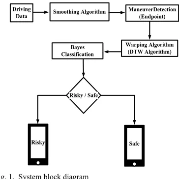
II. THEORYAND STAGES OF SYSTEM DIAGRAM
As sketched in Fig. 1, the first step in our design is the data acquisition and preprocessing of the data via classifier is applied to identify risky of safe driving habit. Details of these steps are given in the following sections.
A. Endpoint Detection
In order to detect the current event, our algorithm continuously acquires data from the accelerometer, gyroscope, and magnetometer. We conjecture risky events occur when there are sharp or sudden maneuvers, unsafe left or right turns, lane departures, and sudden braking or speed-up. These events may result in potential risks for driver, passengers and pedestrians. The reason for these
maneuvers may be related to drivers’ present
mood/behavior such as aggressive driving, drowsiness, inattention and driving while intoxicated.
The signal that relates to such events is estimated by end-point detection algorithm. As an example we show the start and end points of left and right turns in Figure 2. The detection of left turn, right turn, lane departure, acceleration with throttle and deceleration by braking is performed by matching training templates for these events with the test data. The templates for these events are
manually selected and labeled as safe driving habits. Given the event templates, the analysis is continuously performed while acquiring the input data during driving sessions.
In the end point detection, the algorithm works by organizing the samples using windowing method. For each window, the energy of samples lying within is estimated by;
E= (1)
where E is the energy for one window, s[k] is the data
residing in each window, is the mean value of the data
for the window, is the standard deviation of these data
and m is the window size. The threshold for the estimation
problem is determined empirically from the observed energy patterns in the training data. The energy scores beyond the threshold range are eliminated. This process provides us with the signal portion that will be processed for a potential event.
B. DTW Algorithm
Once the start and end points of a potential event is detected, our system accommodates differences between the training and test event durations using the DTW algorithm. In order to estimate the optimal path, DTW proceeds as sketched in Table 1.
TABLEI.
SAMPLEDATATOFINDOPTIMALPATHUSINGDTW
Template
Fig. 1. System block diagram
0.1 0.2 0.3 0.4 0.5 0.6 0.7 0.8 0.9 1
) B-Turn left for the test data
End point
) B-Turn-left for the test data
End Point Start Point
To simplify the pictorial representation we divide the speed by 10. Therefore 6 refers to 60 km in the Table 1. Here the left column represents the data from the template event ordered in top-down direction; while bottom line indicates the test-driving data from left to right;
Template event data (x)... 06260033 Test data (y) ... 062600321 Difference for x-y ... 06-44-6030
As shown in Table 1, computing distances for neighboring elements within the matrix created estimate the minimum path. Optimal threshold for the distance between the present and candidate neighbors are empirically determined and is set at 0.05. In DTW
algorithm, two input vectors X={ , ,…, ,…, } and
Y={ , ,…, ,…, } respectively represent the
training and test data. The DTW algorithm starts with computing the Euclidean distance between X and Y vectors in order to compute the optimal similarity between them;
D(i,j)= (2)
The optimal graph path between these temporally ordered templates, hence, the distances for every element in D matrix of mxn size are calculated. Minimum path to
neighbor element is saved in matrix given by;
(3)
B. Behavior Classification Algorithm
The statistical classification algorithm used in this study adopts Bayesian inference. We assume the existence of two classes related to safe and unsafe driving habits. Mathematical expression for proposed classification is given by;
(4)
where is the class, s is observations for driving events.
Given the priori probabilities of these two classes for driving events, the system output can be obtained by comparing the posteriori probabilities;
P( |s) > P( |s) → Driving at risk (5.a)
P( |s) <= P( |s) → Driving safe (5.b)
D. iPhone Accelerometer and Gyroscope Sensor
In our design, we used the sensors available in iPhone. We should note that current smart phones generally provide these sensory data and our implementation is not iPhone specific. There are several sensors located in iPhone. Among others, we use the gyroscope and accelerometer data in this study.
In our context, accelerometer sensor data gives the
amount of acceleration applied to the vehicle in the (x, y,
z) planes. The accelerometer data also provides the
position and speed information of the vehicle. On the other hand, the gyroscope measurements provide reliable information regarding the lane departure and turning events.
The accelerometer provides data in the range of [−1,1]
and the data from gyroscope range between [−180° 180°].
In order to emphasize sudden variations in the raw data, we first apply a high pass filter to it by;
=accel.(x,y,z)*filtsbt+ *(g-filtsbt)*(accel.(x,y,z))(6)
where “accel.(x,y,z)” represents the data obtained by
accelerometer; g is the gravitational acceleration which is
constant rate, g=1.0, and filtsbt is the frequency rate for
the gravity.
III. EXPERIMENTAL RESULTS
survey result 2 drivers have been estimated as unsafe and 8 drivers as safe. Consequently, we have assigned 0.2 to
P( ) for prior unsafe probability and 0.8 to P ( ) for
prior safe driving probability rate at first. In the experiments, departure point is chosen as the Firat (Euphrates) Technology Development Center and the arrival point is chosen as the Organized-Industrial-Zone. In all the experiments, we have observed lane change, instant acceleration and deceleration, left and right turns, as well as abnormal driving habits.
The vehicle reference frame for the car is defined as has been done considering described reference frames. Below, we detail our results in the order of the processing steps applied to the acquired sensory data.
Once the template and input data warping is performed, the Bayesian classifier is used to make the event type decision based on the maximum a posteriori estimate across different events, and also we can estimate the system output as;
System Output=P( | Steering Angle Bayes Classification, Acceleration Bayes Classification, Slowdowns Bayes Classification, Lane Change Bayes Classification)
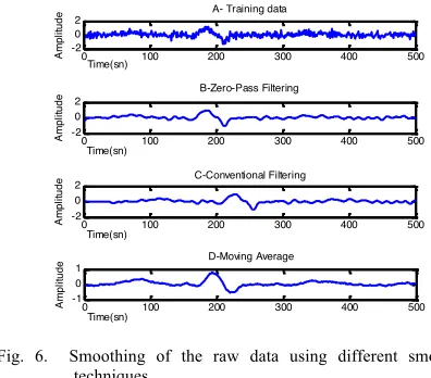
Experimental setup is given in Figure 5. The accelerometer data from the iPhone sensors is first smoothed prior to analyzing the speed of the vehicle. As shown in Figure 6, we applied various smoothing filters to the raw sensor data for eliminating the effect of noise. As seen in the figure we observe that the effect of noise is minimum for the moving average filter. After this step, the endpoints of the events of interest are detected on the smoothed signal to find the range of action.
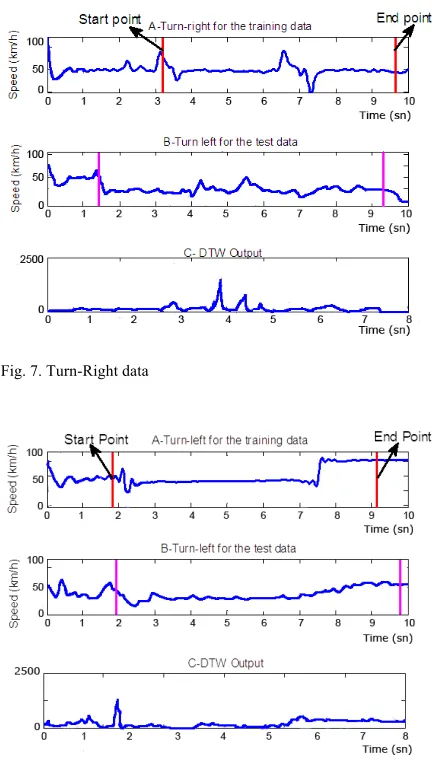
We present detected end-points for an exemplar turn left event in Figure 7. The training and test data in the proposed system is prepared as follows;
Step 1. An experienced driver is asked to prepare training templates of various events, such as the safe turning-left action.
Step 2. A volunteer driver is asked to drive the car without describing the system to reduce the effect of bias. The data is analyzed to detect events. The events are classified using the trained Bayesian classifier.
Departure
Fig. 4.Vehicle and iPhone coordinate system.
Vehicle Data
Fig. 5. Utilizing iPhone sensors in the proposed system
Opposite to the signals in Figure 7, which exemplify turn-right driving pattern and are taken by iPhone sensor, turn-left signals are shown in Figure 8. The visualization of the safe and unsafe driving pattern of Figures 7 and 8 is given in Figure 9.
We show the results of the Bayes classification in Figure 10. The final output of the classification is recorded as safe or unsafe driving. Variables used in the Bayesian classification step for the proposed system and their definitions are given in Table II.
Table III has been designated by considering some of related works. Therefore, we can conclude that process duration of Bayesian classification is less than the others, and it has greater success rate. In the experiments, 14 out of 15 drivers involved in the test-driving have been classified as correct.
Fig. 7. Turn-Right data
Fig. 8. Turn-Left event data
(a) Safe driving (b) Unsafe driving
Fig. 9. A sample safe/unsafe driving event scenes for right turn
TABLEII.
BAYES’VARIABLESFORPROPOSEDSYSTEM
Events (s) Represented
Variable
Correspondent Situation
1. Steering Wheel Angle Unsafe
Safe
2. Acceleration Unsafe
Safe
3. Slowdown Unsafe
Safe
4. Lane Change Unsafe
Safe
0 500 1000 1500 2000 2500
0 0.5 1
Time(sn)
N
o
rm
.
sp
e
e
d A-Training data
0 500 1000 1500 2000 2500
0 0.5
Time(sn)
p
(a
|s)
B-Bayesian P(a|s) Unsafe Status Chance
0 500 1000 1500 2000 2500
0 0.5 1
Time(sn)
p
(n
|s)
C-Bayesian P(n|s) Safe Status Chance
Fig. 10. Bayesian classification using steering wheel, (a) Template data for the system
(b) P(a|s) unsafe probability obtained by the result of Bayesian classification process.
(c) P(n|s) safe driving probability obtained by the result of Bayesian classification.
TABLEIII.
PERFORMANCECOMPARISONFORDIFFERENTMETHODS
Method Time (second) Correctly Classified Instances (%)
Random Forest [10] 24.4 93.0
J48 [10] 78.8 90.6
HMM [2] N/A 85.7
Bayes Classification (Proposed)
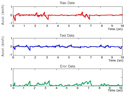
The instant error estimation is obtained by;
(8)
Ground truth, observation signal and the error signal, respectively, are shown in Fig. 11.
IV. CONCLUSION
In this paper we have investigated driver behavior as safe or unsafe using optimal path detection algorithm and Bayesian classification. Event data are acquired by smart phone sensors, which are accelerometer, gyroscope and magnetometer. And also, we have compared the proposed algorithm to the other methods used. Consequently, Bayesian classification output for experiments have showed that the event type and its safe/unsafe driving style have been found as correct for 14 drivers out of 15.
On the other hand, both computational and
implementation cost of the proposed method are promising in compared to the other methods.
In the future work, we are planning to combine driver ambulatory data, CAN bus data from the car and environmental data. Therefore, we will investigate the impact of different driving parameters on driver mood.
REFERENCES
[1] D. A. Johnson and M. M. Trivedi, “Driving Style Recognition Using a Smartphone as a Sensor Platform,” IEEE Transactions On Intelligent Transportation Systems, pp. 1609-1615, 2011.
[2] N. Oliver and A. P. Pentland, “Graphical Models of Driver Behavior Recognition and Prediction in a Smart Car,” IEEE of Intelligent Vehicles Symposium, Cambridge, pp. 7 -12, 2000.
[3] H. Malik and A. Rakotonirainy, “The Need Of Intelligent Driver Training Systems For Road Safety,” In: 19th International Conference on Systems Engineering (ICSENG 2008), Las Vegas, USA., pp. 183-188, 2008. [4] D. Mitrovid, “Driving Event Recognition by Hidden
Markov Models,” 4th International Conference on Telecommunication in Modern Satellite, Cable and Broadcasting Services, vol. 1, pp. 110-113,1999.
[5] D. Mitrovid, “Reliable Method for Driving Events Recognition,” IEEE Transactions On Intelligent Transportation Systems, vol. 6, pp. 198-205, 2005. [6] J. A. Healey and R. W. Picard, “Detecting Stress During
Real-World Driving Tasks Using Physiological Sensors,” IEEE Transactions On Intelligent Transportation Systems, vol. 6, pp. 156-166, 2005.
[7] H. Sakoe and S. Chiba, “Dynamic programming algorithm optimization for spoken word recognition,” IEEE Transactions on Acoustics, Speech and Signal Processing, vol. 26, pp. 43-49, 1978.
[8] L. Rabiner and Biing-Hwang Juang,”Fundamentals of Speech recognition,” New Jersey: Prentice-Hall International, pp. 1-507, 1993.
[9] J. Dai, J. Teng, X. Bai, Z. Shen and D. Xuan, “Mobile Phone Based Drunk Driving Detection,” IEEE Pervasive Computing Technologies for Healthcare Pervasive Health 4th International Conference, pp. 1–8, 2010.
[10]J. C. Magaña and M. M. Organero, “Artemisa: Using an Android device as an Eco-Driving assistant,” Journal of Selected Areas in Mechatronics (JMTC), June Edition, pp. 1-8, 2011.
[11]J. Pauwelussen and P.J. Feenstra, “Driver Behavior Analysis During Activation and Deactivation in a Real Traffic Environment,”IEEE Transactions on Intelligent Transportation Systems, vol. 11, pp. 329-338, 2010. [12]A. Tawari and M.M. Trivedi, “Audio Visual Cues in
Driver Affect Characterization: Issues and Challenges in Developing Robust Approaches,” The 2011 International Joint Conference onNeural Networks (IJCNN), pp. 2997 – 3002, 2011.
[13]R.W. Picard, E. Vyzas and J. Healey, “Toward machine emotional intelligence: analysis of affective physiological state, ”IEEE Transactions on Pattern Analysis and Machine Intelligence, vol. 23, pp. 1175 – 1191, 2001.
[14]A. Riener, “Subliminal Persuasion and Its Potential for Driver Behavior Adaptation,” IEEE Transactions On Intelligent Transportation Systems, pp. 1-10, 2012. [15]D.I. Katzourakis, E. Velenis, D. A. Abbink, R. Happee and
E. Holweg, “Race-Car Instrumentation for Driving Behavior Studies,” IEEE Transactions on Instrumentation and Measurement, vol. 61, pp. 462 – 474, 2012.