MODELLING CARRYING CAPACITY FOR THE THANDA PRIVATE GAME
RESERVE, SOUTH AFRICA USING LANDSAT 8 MULTISPECTRAL DATA
Z. Oumar1,*, J.O. Botha2, E. Adam1, C. Adjorlolo3
1University of Witwatersrand, School of Geography, Archaeology and Environmental Studies, Private Bag 3, Witwatersrand
2050, South Africa - [email protected] , [email protected]
2Department of Agriculture and Rural Development, Private Bag X9059, Pietermaritzburg 3200, South Africa
3South African National Space Agency (SANSA), SANSA Earth Observation, P.O. Box 484, Silverton 0127, South Africa -
KEY WORDS: Carrying capacity, Landsat 8, PLS regression, Broadband indices
ABSTRACT:
Rangelands which consist of grasslands, shrublands and savannahs are used by wildlife for habitat and are the main source of forage for livestock. The assessment and monitoring of rangeland condition is one of the most important factors for rangeland scientists in order to calculate the carrying capacity of livestock with consideration for coexisting wildlife. This study assessed the potential of Landsat 8 multispectral bands and broadband vegetation indices to model woody vegetation parameters such as tree equivalents (TE) and total leaf mass (LMASS) for the Thanda Private Game Reserve using partial least squares regression (PLSR). The PLSR model predicted TE with an R2 value of 0.76 and a root mean square error (RMSE) of 1411 TE/ha using an independent test dataset. LMASS was predicted with an R2 value of 0.67 and a RMSE of 853 kg/ha on an independent test dataset. The predictive models were then inverted to map TE and LMASS over the study area. The modelled TE and LMASS layers were integrated with conventional grazing and browse capacity models to map carrying capacity for the Game Reserve. The study indicates the potential of Landsat 8 multispectral data in carrying capacity modelling. The result is significant for rangeland monitoring in Southern Africa using remote sensing technologies.
1. INTRODUCTION
Rangelands are important natural ecosystems consisting of grasslands and savannahs which provide habitat for wildlife and grazing areas for domestic stock (Hunt et al., 2003). The management and monitoring of this critical resource is essential to its sustainability. Rangeland degradation can be defined as a reduction or loss in grassland productivity due to either over utilization of the herbaceous layer or the encroachment of woody plants (Rutherford and Powrie, 2010) and can be caused by poor landuse management practices (Hoffman and Todd, 2000). Up to date rangeland information linked to carrying capacity is required by rangeland scientists in order to optimally manage rangeland resources (Adjorlolo and Botha, 2015). Traditional rangeland management approaches relies mainly on expert judgment based on a limited number of measured observations whereby the data is characterized by small sample sizes of restricted spatial extent in heterogeneous landscapes (Booth and Tueller, 2003). Remote sensing technologies provide the opportunity to monitor rangeland parameters at landscape
level due to advances in sensor development and well tested algorithms (Hunt et al., 2003). However the integration of conventional grazing and browse capacity models and remote sensing datasets has been limited to a few studies (Adjorlolo and Botha, 2015, Espach et al., 2009, Long et al., 2010). This lack of integration is largely due to the high costs involved in field data collection, inconsistent techniques for calculating grazing and browse capacity (Adjorlolo and Botha, 2015) and the cost and availability of satellite datasets. With the advent of the new Landsat 8 sensor which offers freely available imagery at a temporal resolution of 16 days, rangeland scientists have the opportunity to monitor and assess rangeland health on a regular basis. Furthermore, robust indices and algorithms developed from the Landsat 8 sensor and integration with carrying capacity modelling has not been tested to the best of our knowledge. This study aims to assess the potential of Landsat 8 multispectral bands and broadband vegetation indices in modelling TE and LMASS as inputs into grazing and browse capacity models at Thanda Private Game Reserve.
2. STUDY AREA
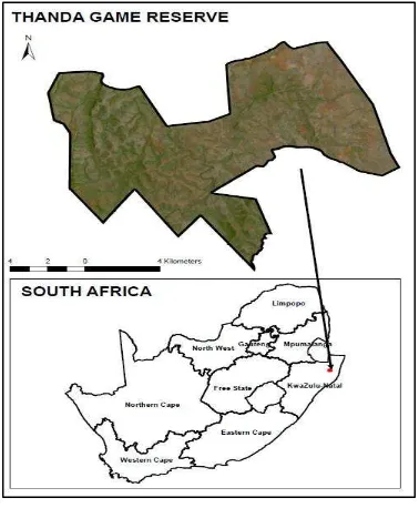
The study area is located in the Umkhanyakude district municipality of South Africa and covers an area of approximately 13 668 ha. The Thanda Private Game Reserve receives an average rainfall of about 647 mm per anum (Schulze and Lynch, 2007) along an altitudinal gradient that ranges from 140 to 660m above sea level (Schulze and Horan, 2007). The mean annual temperature of the reserve is 20 degrees Celsius (Schulze and Maharaj,
Figure 1. Study area
3. METHODS 3.1 Field sampling
Woody plant sampling was carried out in February and March 2016 whereby 40 stratified random sampling plots
where generated across the reserve. The sampling plots were characterized by two parallel 25m x 2.5m belt transects along opposite sides of the sampling plot. All woody plants within the belt transect were identified and their growth form was characterized. Measurements were made using a ranging rod and consisted of:
Maximum tree height (m)
Height of the maximum canopy (m)
Height of minimum canopy (m)
Maximum canopy diameters (m)
Minimum canopy diameters (m)
The field measurements were analysed using the biomass estimates from canopy volume (BECVOL) model (Smit, 1996) which was developed for assessing relationships between woody plant dimensions and its aboveground biomass. The BECVOL model generates several woody plant outputs consisting of tree equivalents (TE) per hectare and leaf mass (LMASS) in kilograms at different height classes (Adjorlolo and Botha, 2015). The TE and LMASS data for each plot were then integrated with Landsat 8 spectral data to model TE and LMASS across the reserve.
3.2 Landsat 8 imagery
One scene of Landsat 8 multispectral data covering the reserve with an image pass of 2nd February 2016 was acquired from the United States geological Survey (USGS) earth explorer website. The scene was atmospherically corrected to top of atmosphere reflectance using the FLAASH (Fast Line-of-Sight Atmospheric Analysis of Spectral Hypercubes) algorithm built in the ENVI (Environment for Visualising Images: ENVI, 2006) software. Landsat 8 Operational Land Imager (OLI) and Thermal Infrared Sensor (TIRS) data consists of 9 spectral bands. Bands 10 and 11 are the thermal bands which are used for surface temperature estimates and are collected at 100 metres (USGS, 2014). The spectral and spatial resolution of the Landsat 8 sensor is shown in Table 1.
Table 1. Spectral and spatial resolution of Landsat 8
3.3 Vegetation Indices
Two commonly used broadband vegetation indices (Equation 1 and 2) were calculated from the Landsat 8 imagery. The Normalized Difference Vegetation Index (NDVI) (Rouse et al., 1973) uses the red and near-infrared band of the electromagnetic spectrum to assess changes in vegetation phenology as it uses the highest absorption and reflectance of the chlorophyll region. The Simple Ratio (SR) (Jordan, 1969) is the ratio of the near-infrared and red bands and is used to assess changes in green vegetation cover.
NDVI = � −� + (1)
SR = � (2)
3.4 Modelling TE and LMASS using partial least squares regression and Landsat 8 data
The reflectance data from the Landsat 8 bands and the two broadband vegetation indices were extracted from the 40 field sampling plots and input into a partial least squares regression algorithm in order to model TE and LMASS across the study area. The forty sampling plots were randomly divided in two sets whereby 50% of the dataset was used for training the model and the remaining 50% was used for validation. PLS regression is a bilinear calibration method which reduces a large number of measured collinear variables to a few non-correlated latent variables or factors (Geladi and Kowlski, 1986, Cho et al., 2007). The PLS model finds a few PLS factors that explain a large amount of variation in both the response and predictor variables (Tobias, 1995). The PLS model is formulated as:
Bands Spectral
Range (micrometres)
Spatial Resolution
(metres) 1- Coastal aerosol 0.43-0.45 30
2- Blue 0.40-0.51 30
3- Green 0.53-0.59 30
4- Red 0.64-0.67 30
5- NIR 0.85-0.88 30
6- SIR1 1.57-1.65 30
7- SIR2 2.11-2.29 30
8-Panchromatic 0.50-0.68 15
9-Cirrus 1.36-1.38 30
10-TIR 1 10.60-11.19 100
Y = XB + E, (3)
where Y is the matrix containing the response variable (TE and LMASS), X is the matrix containing the predictor variables (Landsat 8 bands and vegetation indices), B is the matrix containing the regression coefficients, and E is the matrix of the residuals (Cho et al., 2007). PLS regression was performed using the training dataset and v-fold cross validation was used to select the optimal number of factors and was repeated 10 folds (Hoskuldsson, 2003). The cross validation estimates the predictive residual sum of squares (PRESSs) statistic, for each factor and selects the models with least error. The PRESS is calculated for the final model with the estimated number of significant factors and is often re-expressed as Q2 (the cross validated R2) (Wold et al., 2001). The cross validated PLS model was then extrapolated to map TE and LMASS across the study area. The predictive accuracy of the modelled map was assessed using the coefficient of determination (R2) and the root mean square error (RMSE) on the independent 50% test dataset.
3.5 Integrating tree equivalents and leaf mass with graze and browse capacity models
The predicted TE layer was input into a grazing capacity equation in order to model grazing capacity across the animal unit (AU) where AU is defined as an animal with a mass of 450 kg, which gains 0.5 kg per day with a digestible energy percentage of 55 % (Meissner, 1993).
The predicted LMASS layer was input into a browse capacity equation in order to model browse capacity over the reserve. Browse capacity was calculated as follows animal requiring 10 kg dry matter per day), ���ℎ is the modelled leaf mass expressed at various height classes, F
is the utilization factor (25 %) based on the percentage of available leaf material utilized by the browsing animal, and P is the phenology factor of (0.744) based on the availability of browse material available throughout the year.
4. RESULTS
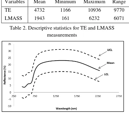
4.1 Tree equivalents and leaf mass measurements Table 2 shows the descriptive statistics for the TE and LMASS measurements. TE ranged from 1166 to 10936 TE/ha and LMASS ranged from 161 to 6232 kg. TE and LMASS showed a range in values and this can be attributed to the variation in vegetation types across the reserve. Figure 2 shows the mean Landsat 8 reflectance for the TE and LMASS plots showing a normal spectral vegetation curve.
Variables Mean Minimum Maximum Range
TE 4732 1166 10936 9770
LMASS 1943 161 6232 6071
Table 2. Descriptive statistics for TE and LMASS measurements
Figure 2. Mean vegetation reflectance from Landsat 8 bands (n=40) showing the mean, 95% upper confidence
limit (UCL), and 95% lower confidence limit (LCL) of the reflectance
4.2 Predicting TE and LMASS with Landsat 8 bands and vegetation indices using PLS regression
Table 3 shows the performance of the PLS regression models in predicting TE and LMASS using the training dataset. The PLS algorithm extracted two factors and predicted TE with and R2 value of 0.54. LMASS was predicted with an R2 value of 0.62 using two PLS factors. The PLS algorithm produces variable importance (VIP) scores that are used to select the relevant predictors in the model according to the magnitude of their values (Chong and Jun 2005, Palermo, Piraino, and Zucht 2009). Figure 3 shows the variable importance in the projection (VIP) for the TE and LMASS.
Figure 3. (a) VIP variables for TE. The red line indicates the VIP cut off value of 1. All predictors above the red
line are significant in the model
Figure 3. (b) VIP variables for LMASS. The red line indicates the VIP cut off value of 1. All predictors above
the red line are significant in the model
4.3 TE and LMASS mapping
The PLS models for TE and LMASS were inverted to map TE and LMASS over the study area. Figure 4 shows the predicted TE and LMASS layers. The performance of the PLS model in predicting TE and LMASS layers was evaluated using the R2 and the RMSE on the independent 50% test dataset (Figure 5).
Figure 4. (a) Predicted TE map
Figure 4. (b) Predicted LMASS map
Figure 5. (a) Performance of the PLS models in predicting TE on the independent test dataset
Figure 5. (b) Performance of the PLS models in predicting LMASS on the independent test dataset
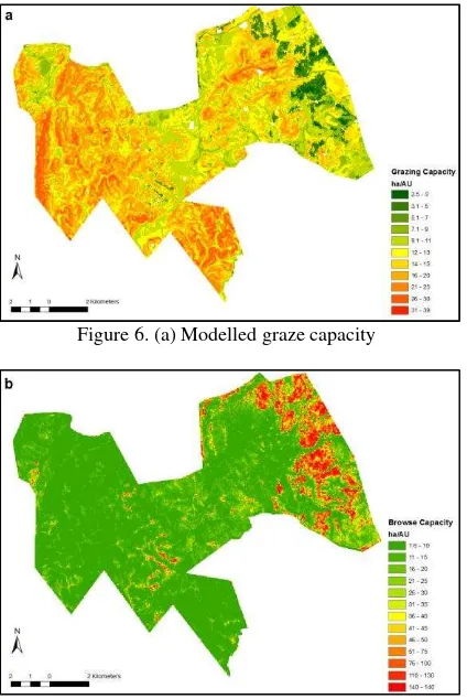
4.4 Integrating TE and LMASS with grazing and browse models
Figure 6. (a) Modelled graze capacity
Figure 6. (b) Modelled browse capacity
5. DISCUSSION
5.1 Modelling TE and LMASS with Landsat 8 bands and indices
TE and LMASS were modelled with relatively high accuracies of 0.76 and 0.67 on an independent test dataset using PLS regression. The TE had a RMSE of 1411 TE/Ha and the LMASS had a RMSE of 853 kg/ ha. The VIP scores for TE showed that the Shortwave Infrared band 2 was the best predictor in the model with a VIP score of 1.28 followed by the NDVI with a score of 1.23 and the SR index with a score of 1.18. The VIP scores for the LMASS indicated that the best predictor in the model was the SR index with a score of 1.26 followed by the shortwave infrared band 2 with a score of 1.20 and then the NDVI with a score of 1.20. The shortwave infrared region is sensitive to vegetation water content as it has strong water absorption bands at 1940 and 2500 nm (Carter, 1991, Datt, 1999). The NDVI index which is based on the near-infrared region is widely used to assess vegetation properties and is sensitive to changes in plant growth and vigour (Penuelas and Filella, 1998). The modelled result is comparable to the earlier work done by Adjorlolo and Botha (2016) who predicted TE with an R2 value of 0.55 and LMASS with an R2 value of 0.64 using SPOT 5 data and the random forest algorithm. Adjorlolo and Botha (2016) found that the modelled TE and LMASS improved the detail in the grazing and browse capacity layers as compared to the expert opinion and field surveyed method which generalized the graze and browse
outputs. This is also true for the Landsat 8 derived product whereby the PLS algorithm identified significant factors which explain most of the variation in the dataset in predicting TE and LMASS. The study indicates the potential of broadband vegetation indices derived from the Landsat 8 sensor to spatially model woody vegetation properties across the reserve.
5.2 Integrating TEs and LMASS to model grazing and browsing across the reserve
The setting of stocking rates is one of the most important decisions for rangeland managers (Hunt et al., 2003) and this is often achieved through field measurements which indicate the composition and density of herbaceous and woody plant biomass at a single point in time and at low spatial distribution (Espach et al., 2010) resulting in the homogenisation of resultant values. The benefit of using remote sensing derived spatial layers in the modelling of carrying capacity at finer scales translates into more accurate stocking rate estimates and improves the potential for detailed home range analysis of high value ungulate species. The relatively coarser pixel resolution of Landsat 8 compared to Spot 5 and Spot 6 renders it less sensitive to noise emanating from structural heterogeneity in savannah dominated landscapes. Furthermore Landsat 8 data has the additional benefit of been freely available and the higher temporal availability allows for investigating temporal changes in vegetation structure and condition by researchers in governmental and non-profit agencies. Accurate plant measurements are required on a regular basis and this is impractical in large areas due to the effort, time and expenses involved. Satellite imagery is a more practical and efficient method of acquiring variation in biomass production over time (Ganzin et al., 2005). The integration of multi temporal imagery consisting of broadband vegetation indices and conventional graze and browse capacity models allows for carrying capacity to be modelled on a seasonal basis. This study showed the potential of integrating modelled TE and LMASS data derived from the Landsat 8 sensor to model graze and browse capacity across the reserve. With the temporal resolution of the Landsat 8 sensor been every 16 days, rangeland managers have the opportunity to monitor the rangelands on a more frequent basis.
6. CONCLUSION
REFERENCES
Adjorlolo, C. and Botha, J.A. 2015. Integration of remote sensing and conventional models for modelling grazing/browsing capacity in southern African savannas,
Journal of Applied Remote Sensing, 9, pp. 1-16.
Booth, D.T., and Tueller, P.T. 2003. Rangeland monitoring using remote sensing, Arid Land Research and Management, 17, pp. 455-467.
Camp, K.G.T and Hardy, M.B. 1999. Veld Condition Assessment, KwaZulu-Natal, Department of Agriculture, Cedara, Pietermaritzburg.
Carter, G.A., 1991. Primary and secondary effects of water content on the spectral reflectance of leaves.
American Journal of Botany, 78 (7), pp. 916-924.
Cho, M. A., Skidmore, A., Corsi, F., Van Wieren, S.E. and Sobhan, I. 2007. Estimation of Green Grass/Herb Biomass from Airborne Hyperspectral Imagery Using Spectral Indices and Partial Least Squares Regression,
International Journal of Applied Earth Observation and Geoinformation 9, pp. 414–24.
Chong, I., and Jun, C. 2005. Performance of Some Variable Selection Methods When Multicollinearity Is Present, Chemometrics and Intelligent Laboratory Systems, 78, pp. 103–12.
Datt, B., 1999. Remote sensing of water content in Eucalyptus leaves. Australian Journal of Botany, 47, pp. 909-923.
ENVI, 2006. Environment for Visualising Images. Release 4.3. ITT industries, Inc, Boulder, USA.
Espach, C., Lubbe, L.G. and Ganzin, N. 2009. Determining grazing capacity in Namibia with the aid of remote sensing, African Journal of Range and Forage Science, 26(3), pp. 133-138.
Ganzin, N., Coetzee, M.C., Rothauge, A. and Fotsing, J.M. 2005. Rangeland Resources Assessment with Satellite Imagery: An Operational Tool for National Planning in Namibia, Geocarto International, 20 (3), pp. 33-42.
Geladi, P. and Kowlski, B. 1986. Partial Least-Squares Regression: A Tutorial. Analytica Chimica Acta, 185, pp. 1–17.
Han, J.G., Zhang, Y.J., Wang, C.J., Bai, W.M., Wang, Y.R., Han, G.D., Li, L.H. 2008. Rangeland degradation and restoration management in China, The Rangeland Journal, 30, pp. 233-239.
Hoffman, M. and Todd, S., 2000. A national review of land degradation in South Africa: the influence of biophysical and socio-economic factors, Journal of Southern African Studies, 26 (4), pp. 743-758.
Hoskuldsson, A. 2003. Analysis of Latent Structures in Linear Models, Journal of Chemometrics, 17, pp. 630–45.
Hunt, E.R., Everitt, J.H., Ritchie, J.C., Moran, M.S., Booth, D.T., Anderson, G.L., Clark, P.E., Seyfried, and M.S. 2003. Applications and research using remote
sensing for rangeland management, Photogrammetric Engineering and Remote Sensing, 69 (6), pp. 675-693.
Jordan, C.F. 1969. Derivation of leaf area index from quality of light on the forest floor, Ecology, (50), pp. 663-666.
Long, Y.U., Li, Z., Wei, L., Hua-Kun, Z. 2010. Using Remote Sensing and GIS Technologies to Estimate Grass Yield and Livestock Carrying Capacity of Alpine Grasslands in Golog Prefecture, China, Pedosphere, 20 (3), pp. 342-351.
Meissner, H.H. 1993. Carrying capacity as estimated by the animal unit and biomass methods: pros and cons, in
Proceedings of the Workshop on Determining Grazing Norms.
Palermo, G., Piraino, P. and Zucht, H. 2009. Performance of PLS Regression Coefficients in Selecting Variables for Each Response of a Multivariate PLS for Omics-Type Data, Advances and Applications in Bioinformatics and Chemistry, 2, pp. 57–70.
Penuelas, J. and Filella, L. 1998. Visible and near-infrared reflectance techniques for diagnosing plant physiological status, Trends in plant science, 3(4), pp. 151-156.
Rouse, J.W., Haas, R.H., Schell, J.A. and Deering, D.W. 1973. Monitoring Vegetation Systems in the Great Plains with ERTS, Third ERTS Symposium. NASA, Washington, DC, pp. 309-317.
Rutherford, M. and Powrie, L. 2010. Severely degraded rangeland: Implications for plant diversity from a case study in Succulent Karoo, South Africa, Journal of Arid Environments, 74 (6), pp. 692-701.
Schulze, R.E. and Horan, M.J.C. 2007. Altitude and Relative Relief, In: Schulze, RE (ed.), South African Atlas of Climatology and Agrohydrology, Water Research Commission, Pretoria, RSA.
Schulze, R.E. and Lynch, S.D. 2007. Annual Precipitation, In: Schulze, RE (ed.), South African Atlas of Climatology and Agrohydrology, Water Research Commission, Pretoria, RSA.
Schulze, R.E. and Maharaj, M. 2007. Mean Annual Temperature, In: Schulze, RE (ed.), South African Atlas of Climatology and Agrohydrology, Water Research Commission, Pretoria, RSA.
Scott-Shaw, C.R. and Escott, B.J. 2011. “KwaZulu-Natal provincial pre-transformation vegetation type map - 2011, unpublished GIS coverage (kznveg05v2_1_11_wll.zip),” Biodiversity Conservation. Planning Division, Ezemvelo KZN Wildlife, Cascades, Pietermaritzburg.
Smit, G.N. 2009. Calculation of Grazing Capacity and Browse Capacity for Game Species, University of the Free State, Bloemfontein.