For your convenience Apress has placed some of the front
matter material after the index. Please use the Bookmarks
and Contents at a Glance links to access them.
Contents at a Glance
About the Author ...
xv
About the Technical Reviewer ...
xvii
Acknowledgments ...
xix
Preface ...
xxi
Chapter 1: Introduction
■
...
1
Chapter 2: Digital Video Compression Techniques
■
...
11
Chapter 3: Video Coding Standards
■
...
55
Chapter 4: Video Quality Metrics
■
...
101
Chapter 5: Video Coding Performance
■
...
161
Chapter 6: Power Consumption by Video Applications
■
...
209
Chapter 7: Video Application Power Consumption on
■
Low-Power Platforms ... 259
Chapter 8: Performance, Power, and Quality Tradeoff Analysis
■
...297
Chapter 9: Conclusion
■
...
321
Appendix A: Appendix
■
...
329
Introduction
Over the past decade, countless multimedia functionalities have been added to mobile devices. For example, front and back video cameras are common features in today’s cellular phones. Further, there has been a race to capture, process, and display ever-higher resolution video, making this an area that vendors emphasize and where they actively seek market differentiation. These multimedia applications need fast processing capabilities, but those capabilities come at the expense of increased power consumption. The battery life of mobile devices has become a crucial factor, whereas any advances in battery capacity only partly address this problem. Therefore, the future’s winning designs must include ways to reduce the energy dissipation of the system as a whole. Many factors must be weighed and some tradeoffs must be made.
Granted, high-quality digital imagery and video are significant components of the multimedia offered in today’s mobile devices. At the same time, there is high demand for efficient, performance- and power-optimized systems in this resource-constrained environment. Over the past couple of decades, numerous tools and techniques have been developed to address these aspects of digital video while also attempting to achieve the best visual quality possible. To date, though, the intricate interactions among these aspects had not been explored.
The Key Concepts
This section deals with some of the key concepts discussed in this book, as applicable to perceived visual quality in compressed digital video, especially as presented on contemporary mobile platforms.
Digital Video
The term video refers to the visual information captured by a camera, and it usually is applied to a time-varying sequence of pictures. Originating in the early television industry of the 1930s, video cameras were electromechanical for a decade, until all-electronic versions based on cathode ray tubes (CRT) were introduced. The analog tube technologies were then replaced in the 1980s by solid-state sensors, particularly CMOS active pixel sensors, which enabled the use of digital video.
Early video cameras captured analog video signals as a one-dimensional, time-varying signal according to a pre-defined scanning convention. These signals would be
transmitted using analog amplitude modulation, and they were stored on analog video tapes using video cassette recorders or on analog laser discs using optical technology. The analog signals were not amenable to compression; they were regularly converted to digital formats for compression and processing in the digital domain.
Recently, use of all-digital workflow encompassing digital video signals from capture to consumption has become widespread, particularly because of the following characteristics:
It is easy to record, store, recover, transmit, and receive, or to •
process and manipulate, video that’s in digital format; it’s virtually without error, so digital video can be considered just another data type for today’s computing systems.
Unlike analog video signals, digital video signals can be •
compressed and subsequently decompressed. Storage and transmission are much easier in compressed format compared to uncompressed format.
With the availability of inexpensive integrated circuits, high-speed •
communication networks, rapid-access dense storage media, advanced architecture of computing devices, and high-efficiency video compression techniques, it is now possible to handle digital video at desired data rates for a variety of applications on numerous platforms that range from mobile handsets to networked servers and workstations.
Video Data Compression
It takes a massive quantity of data to represent digital video signals. Some sort of data compression is necessary for practical storage and transmission of the data for a plethora of applications. Data compression can be lossless, so that the same data is retrieved upon decompression. It can also be lossy, whereby only an approximation of the original signal is recovered after decompression. Fortunately, the characteristic of video data is such that a certain amount of loss can be tolerated, with the resulting video signal perceived without objection by the human visual system. Nevertheless, all video signal-processing methods and techniques make every effort to achieve the best visual quality possible, given their system constraints.
Note that video data compression typically involves coding of the video data; the coded representation is generally transmitted or stored, and it is decoded when a decompressed version is presented to the viewer. Thus, it is common to use the terms
compression/decompression and encoding/decoding interchangeably. Some professional video applications may use uncompressed video in coded form, but this is relatively rare. A codec is composed of an encoder and a decoder. Video encoders are much more complex than video decoders are. They typically require a great many more signal-processing operations; therefore, designing efficient video encoders is of primary importance. Although the video coding standards specify the bitstream syntax and semantics for the decoders, the encoder design is mostly open.
Chapter 2 has a detailed discussion of video data compression, while the important data compression algorithms and standards can be found in Chapter 3.
Noise Reduction
Although compression and processing are necessary for digital video, such processing may introduce undesired effects, which are commonly termed distortions or noise. They are also known as visual artifacts. As noise affects the fidelity of the user’s received signal, or equivalently the visual quality perceived by the end user, the video signal processing seeks to minimize the noise. This applies to both analog and digital processing, including the process of video compression.
In digital video, typically we encounter many different types of noise. These include noise from the sensors and the video capture devices, from the compression process, from transmission over lossy channels, and so on. There is a detailed discussion of various types of noise in Chapter 4.
Visual Quality
Visual quality is a measure of perceived visual deterioration in the output video compared to the original signal, which has resulted from lossy video compression techniques. This is basically a measure of the quality of experience (QoE) of the viewer. Ideally, there should be minimal loss to achieve the highest visual quality possible within the coding system.
Note that because of compression, the artifacts found in digital video are fundamentally different from those in analog systems. The amount and visibility of the distortions in video depend on the contents of that video. Consequently, the measurement and evaluation of artifacts, and the resulting visual quality, differ greatly from the traditional analog quality assessment and control mechanisms. (The latter, ironically, used signal parameters that could be closely correlated with perceived visual quality.)
Given the nature of digital video artifacts, the best method of visual quality assessment and reliable ranking is subjective viewing experiments. However, subjective methods are complex, cumbersome, time-consuming, and expensive. In addition, they are not suitable for automated environments.
An alternative, then, is to use simple error measures such as the mean squared error
(MSE) or the peak signal to noise ratio (PSNR). Strictly speaking, PSNR is only a measure of the signal fidelity, not the visual quality, as it compares the output signal to the input signal and so does not necessarily represent perceived visual quality. However, it is the most popular metric for visual quality used in the industry and in academia. Details on this use are provided in Chapter 4.
Performance
Video coding performance generally refers to the speed of the video coding process: the higher the speed, the better the performance. In this context, performance optimization
refers to achieving a fast video encoding speed.
In general, the performance of a computing task depends on the capabilities of the processor, particularly the central processing unit (CPU) and the graphics processing unit
(GPU) frequencies up to a limit. In addition, the capacity and speed of the main memory, auxiliary cache memory, and the disk input and output (I/O), as well as the cache hit ratio, scheduling of the tasks, and so on, are among various system considerations for performance optimization.
Video data and video coding tasks are especially amenable to parallel processing, which is a good way to improve processing speed. It is also an optimal way to keep the available processing units busy for as long as necessary to complete the tasks, thereby maximizing resource utilization. In addition, there are many other performance-optimization techniques for video coding, including tuning of encoding parameters. All these techniques are discussed in detail in Chapter 5.
Power Consumption
A mobile device is expected to serve as the platform for computing, communication, productivity, navigation, entertainment, and education. Further, devices that are
Power management and optimization are the primary concerns for all these existing and new devices and platforms, where the goal is to prolong battery life. However, many applications are particularly power-hungry, either by their very nature or because of special needs, such as on-the-fly binary translation.
Power—or equivalently, energy—consumption thus is a major concern. Power
optimization aims to reduce energy consumption and thereby extend battery life. High-speed video coding and processing present further challenges to power optimization. Therefore, we need to understand the power management and optimization considerations, methods, and tools; this is covered in Chapters 6 and 7.
Video Compression Considerations
A major drawback in the processing, storage, and transmission of digital video is the huge amount of data needed to represent the video signal. Simple scanning and binary coding of the camera voltage variations would produce billions of bits per second, which without compression would result in prohibitively expensive storage or transmission devices. A typical high-definition video (three color planes per picture, a resolution of 1920×1080 pixels per plane, 8 bits per pixel, at a 30 pictures per second rate) necessitates a data rate of approximately 1.5 billion bits per second. A typical transmission channel capable of handling about 5 Mbps would require a 300:1 compression ratio. Obviously, lossy techniques can accommodate such high compression, but the resulting reconstructed video will suffer some loss in visual quality.
However, video compression techniques aim at providing the best possible visual quality at a specified data rate. Depending on the requirements of the applications, available channel bandwidth or storage capacity, and the video characteristics, a variety of data rates are used, ranging from 33.6 kbps video calls in an old-style public switched telephone network to ~20 Mbps in a typical HDTV rebroadcast system.
Varying Uses
In some video applications, video signals are captured, processed, transmitted, and displayed in an on-line manner. Real-time constraints for video signal processing and communication are necessary for these applications. The applications use an end-to-end real-time workflow and include, for example, video chat and video conferencing, streaming, live broadcast, remote wireless display, distant medical diagnosis and surgical procedures, and so on.
Conflicting Requirements
The conflicting requirements of video compression on modern mobile platforms pose challenges for a range of people, from system architects to end users of video applications. Compressed data is easy to handle, but visual quality loss typically occurs with compression. A good video coding solution must produce videos without too much loss of quality.
Furthermore, some video applications benefit from high-speed video coding. This generally implies a high computation requirement, resulting in high energy consumption. However, mobile devices are typically resource constrained and battery life is usually the biggest concern. Some video applications may sacrifice visual quality in favor of saving energy.
These conflicting needs and purposes have to be balanced. As we shall see in the coming chapters, video coding parameters can be tuned and balanced to obtain such results.
Hardware vs. Software Implementations
Video compression systems can be implemented using dedicated application-specific integrated circuits (ASICs), field-programmable gate arrays (FPGAs), GPU-based hardware acceleration, or purely CPU-based software.
The ASICs are customized for a particular use and are usually optimized to perform specific tasks; they cannot be used for purposes other than what they are designed for. Although they are fast, robust against error, yield consistent, predictable, and offer stable performance, they are inflexible, implement a single algorithm, are not programmable or easily modifiable, and can quickly become obsolete. Modern ASICs often include entire microprocessors, memory blocks including read-only memory (ROM), random-access memory (RAM), flash memory, and other large building blocks. Such an ASIC is often termed a system-on-chip (SoC).
FPGAs consist of programmable logic blocks and programmable interconnects. They are much more flexible than ASICs; the same FPGA can be used in many different applications. Typical uses include building prototypes from standard parts. For smaller designs or lower production volumes, FPGAs may be more cost-effective than an ASIC design. However, FPGAs are usually not optimized for performance, and the performance usually does not scale with the growing problem size.
GPU-based hardware acceleration typically provides a middle ground. In these solutions, there are a set of programmable execution units and a few performance- and power-optimized fixed-function hardware units. While some complex algorithms may take advantage of parallel processing using the execution units, the fixed-function units provide fast processing. It is also possible to reuse some fixed-function units with updated parameters based on certain feedback information, thereby achieving multiple passes for those specific units. Therefore, these solutions exhibit flexibility and scalability while also being optimized for performance and power consumption. The tuning of available parameters can ensure high visual quality at a given bit rate.
Tradeoff Analysis
Tradeoff analysis is the study of the cost-effectiveness of different alternatives to determine where benefits outweigh costs. In video coding, a tradeoff analysis looks into the effect of tuning various encoding parameters on the achievable compression, performance, power savings, and visual quality in consideration of the application requirements, platform constraints, and video complexity.
Note that the tuning of video coding parameters affects performance as well as visual quality, so a good video coding solution balances performance optimization with achievable visual quality. In Chapter 8, a case study illustrates this tradeoff between performance and quality.
It is worthwhile to note that, while achieving high encoding speed is desirable, it may not always be possible on platforms with different restrictions. In particular, achieving power savings is often the priority on modern computing platforms. Therefore, a typical tradeoff between performance and power optimization is considered in a case study examined in Chapter 8.
Benchmarks and Standards
The benchmarks typically used today for ranking video coding solutions do not consider all aspects of video. Additionally, industry-standard benchmarks for methodology and metrics specific to tradeoff analysis do not exist. This standards gap leaves the user guessing about which video coding parameters will yield satisfactory outputs for particular video applications. By explaining the concepts, methods, and metrics involved, this book helps readers understand the effects of video coding parameters on the video measures.
Challenges and Opportunities
Several challenges and opportunities in the area of digital video techniques have served as the motivating factors for tradeoff analysis.
The demand for compressed digital video is increasing. With the •
Several international video coding standards are now available to •
address a variety of video applications. Some of these standards evolved from previous standards, were tweaked with new coding features and tools, and are targeted toward achieving better compression efficiency.
Low-power computing devices, particularly in the mobile •
environment, are increasingly the chosen platforms for video applications. However, they remain restrictive in terms of system capabilities, a situation that presents optimization challenges. Nonetheless, tradeoffs are possible to accommodate goals such as preserving battery life.
Some video applications benefit from increased processing •
speed. Efficient utilization of resources, resource specialization, and tuning of video parameters can help achieve faster processing speed, often without compromising visual quality.
The desire to obtain the best possible visual quality on any given •
platform requires careful control of coding parameters and wise choice among many alternatives. Yet there exists a void where such tools and measures should exist.
Tuning of video coding parameters can influence various video •
measures, and desired tradeoffs can be made by such tuning. To be able to balance the gain in one video measure with the loss in another requires knowledge of coding parameters and how they influence each other and the various video measures. However, there is no unified approach to the considerations and analyses of the available tradeoff opportunities. A systematic and in-depth study of this subject is necessary.
A tradeoff analysis can expose the strengths and weaknesses of a •
video coding solution and can rank different solutions.
The Outcomes of Tradeoff Analysis
Tradeoff analysis is useful in many real-life video coding scenarios and applications. Such analysis can show the value of a certain encoding feature so that it is easy to make a decision whether to add or remove that feature under the specific application requirements and within the system restrictions. Tradeoff analysis is useful in assessing the strengths and weaknesses of a video encoder, tuning the parameters to achieve optimized encoders, comparing two encoding solutions based on the tradeoffs they involve, or ranking multiple encoding solutions based on a set of criteria.
Emerging Video Applications
Compute performance has increased to a level where computers are no longer used solely for scientific and business purposes. We have a colossal amount of compute capabilities at our disposal, enabling unprecedented uses and applications. We are revolutionizing human interfaces, using vision, voice, touch, gesture, and context. Many new applications are either already available or are emerging for our mobile devices, including perceptual computing, such as 3-D image and video capture and depth-based processing; voice, gesture, and face recognition; and virtual-reality-based education and entertainment.
These applications are appearing in a range of devices and may include synthetic and/or natural video. Because of the fast pace of change in platform capabilities, and the innovative nature of these emerging applications, it is quite difficult to set a strategy on handling the video components of such applications, especially from an optimization point of view. However, by understanding the basic concepts, methods, and metrics of various video measures, we’ll be able to apply them to future applications.
Summary
Digital Video Compression
Techniques
Digital video plays a central role in today’s communication, information consumption, entertainment and educational approaches, and has enormous economic and
sociocultural impacts on everyday life. In the first decade of the 21st century, the profound
dominance of video as an information medium on modern life—from digital television to Skype, DVD to Blu-ray, and YouTube to Netflix–has been well established. Owing to the enormous amount of data required to represent digital video, it is necessary to compress the video data for practical transmission and communication, storage, and streaming applications.
In this chapter we start with a brief discussion of the limits of digital networks and the extent of compression required for digital video transmission. This sets the stage for further discussions on compression. It is followed by a discussion of the human visual system (HVS) and the compression opportunities allowed by the HVS. Then we explain the terminologies, data structures, and concepts commonly used in digital video compression.
We discuss various redundancy reduction and entropy coding techniques that form the core of the compression methods. This is followed by overviews of various compression techniques and their respective advantages and limitations. We briefly introduce the rate-distortion curve both as the measure of compression efficiency and as a way to compare two encoding solutions. Finally, there’s a discussion of the factors influencing and characterizing the compression algorithms before a brief summary concludes the chapter.
Network Limits and Compression
the ubiquity of the telephone networks meant that the design of new and innovative communication services such as facsimile (fax) and modem were initially inclined toward using these available analog networks. The introduction of ISDN enabled both voice and video communication to engage digital networks as well, but the standardization delay in Broadband ISDN (B-ISDN) allowed packet-based local area networks such as the Ethernet to become more popular. Today, a number of network protocols support transmission of images or videos using wire line or wireless technologies, having different bandwidth and data-rate capabilities, as listed in Table 2-1.
Table 2-1. Various Network Protocols and Their Supported Bit Rates
Network
Bit Rate
Plain Old Telephone Service (POTS) on conventional low-speed twisted-pair copper wiring
2.4 kbps (ITU* V.27†), 14.4 kbps (V.17), 28.8 kpbs (V.34), 33.6 kbps (V.34bis), etc.
Digital Signal 0 (DS 0), the basic granularity of circuit switched telephone exchange
64 kbps
Integrated Services Digital Network (ISDN) 64 kbps (Basic Rate Interface), 144 kbps (Narrow band ISDN)
Digital Signal 1 (DS 1), aka T-1 or E-1 1.5 – 2 Mbps (Primary Rate Interface)
Ethernet Local Area Network 10 Mbps
Broadband ISDN 100 – 200 Mbps
Gigabit Ethernet 1 Gbps
* International Telecommunications Union.
† The ITU V-series international standards specify the recommendations for vocabulary and related subjects for radiocommuncation.
In the 1990s, transmission of raw digital video data over POTS or ISDN was unproductive and very expensive due to the sheer data rate required. Note that the raw data rate for the ITU-R 601 formats1 is ~165 Mbps (million bits per second), beyond the
networks’ capabilities. In order to partially address the data-rate issue, the 15th specialist
group (SGXV) of the CCITT2 defined the Common Image Format (CIF) to have common
picture parameter values independent of the picture rate. While the format specifies many picture rates (24 Hz, 25 Hz, 30 Hz, 50 Hz, and 60 Hz), with a resolution of 352 × 288 at 30 Hz, the required data rate was brought down to approximately 37 Mbps, which would typically fit into a basic Digital Signal 0 (DS0) circuit, and would be practical for transmission.
1ThespecificationwasoriginallyknownasCCIR-601.ThestandardbodyCCIRa.k.a.International
RadioConsultativeCommittee(ComitéConsultatifInternationalpourlaRadio)wasformedin 1927,andwassupercededin1992bytheITURecommendationsSector(ITU-R).
2CCITT(InternationalConsultativeCommitteeforTelephoneandTelegraph)isacommitteeofthe
With increased compute capabilities, video encoding and processing operations became more manageable over the years. These capabilities fueled the growing demand of ever higher video resolutions and data rates to accommodate diverse video applications with better-quality goals. One after another, the ITU-R Recommendations BT.601,3 BT.709,4 and BT.20205 appeared to support video formats with increasingly
higher resolutions. Over the years these recommendations evolved. For example, the recommendation BT.709, aimed at high-definition television (HDTV), started with defining parameters for the early days of analog high-definition television implementation, as captured in Part 1 of the specification. However, these parameters are no longer in use, so Part 2 of the specification contains HDTV system parameters with square pixel common image format.
Meanwhile, the network capabilities also grew, making it possible to address the needs of today’s industries. Additionally, compression methods and techniques became more refined.
The Human Visual System
The human visual system (HVS) is part of the human nervous system, which is managed by the brain. The electrochemical communication between the nervous system and the brain is carried out by about 100 billion nerve cells, called neurons. Neurons either generate pulses or inhibit existing pulses, and result in a variety of phenomena ranging from Mach bands, band-pass characteristic of the visual frequency response, to the edge-detection mechanism of the eye. Study of the enormously complex nervous system is manageable because there are only two types of signals in the nervous system: one for long distances and the other for short distances. These signals are the same for all neurons, regardless of the information they carry, whether visual, audible, tactile, or other.
Understanding how the HVS works is important for the following reasons:
It explains how accurately a viewer perceives what is being •
presented for viewing.
It helps understand the composition of visual signals in terms •
of their physical quantities, such as luminance and spatial frequencies, and helps develop measures of signal fidelity.
3ITU-R.SeeITU-RRecommendationBT.601-5:Studioencodingparametersofdigitaltelevision forstandard4:3andwidescreen16:9aspectratios(Geneva,Switzerland:International TelecommunicationsUnion,1995).
4ITU-R.SeeITU-RRecommendationBT.709-5:ParametervaluesfortheHDTVstandards forproductionandinternationalprogrammeexchange(Geneva,Switzerland:International TelecommunicationsUnion,2002).
It helps represent the perceived information by various attributes, •
such as brightness, color, contrast, motion, edges, and shapes. It also helps determine the sensitivity of the HVS to these attributes.
It helps exploit the apparent imperfection of the HVS to •
give an impression of faithful perception of the object being viewed. An example of such exploitation is color television. When it was discovered that the HVS is less sensitive to loss of color information, it became easy to reduce the transmission bandwidth of color television by chroma subsampling.
The major components of the HVS include the eye, the visual pathways to the brain, and part of the brain called the visual cortex. The eye captures light and converts it to signals understandable by the nervous system. These signals are then transmitted and processed along the visual pathways.
So, the eye is the sensor of visual signals. It is an optical system, where an image of the outside world is projected onto the retina, located at the back of the eye. Light entering the retina goes through several layers of neurons until it reaches the light-sensitive photoreceptors, which are specialized neurons that convert incident light energy into neural signals.
There are two types of photoreceptors: rods and cones. Rods are sensitive to low light levels; they are unable to distinguish color and are predominant in the periphery. They are also responsible for peripheral vision and they help in motion and shape detection. As signals from many rods converge onto a single neuron, sensitivity at the periphery is high, but the resolution is low. Cones, on the other hand, are sensitive to higher light levels of long, medium, and short wavelengths. They form the basis of color perception. Cone cells are mostly concentrated in the center region of the retina, called the fovea. They are responsible for central or foveal vision, which is relatively weak in the dark. Several neurons encode the signal from each cone, resulting in high resolution but low sensitivity.
The number of the rods, about 100 million, is higher by more than an order of magnitude compared to the number of cones, which is about 6.5 million. As a result, the HVS is more sensitive to motion and structure, but it is less sensitive to loss in color information. Furthermore, motion sensitivity is stronger than texture sensitivity; for example, a camouflaged still animal is difficult to perceive compared to a moving one. However, texture sensitivity is stronger than disparity; for example, 3D depth resolution does not need to be so accurate for perception.
Even if the retina perfectly detects light, that capacity may not be fully utilized or the brain may not be consciously aware of such detection, as the visual signal is carried by the optic nerves from the retina to various processing centers in the brain. The visual cortex, located in the back of the cerebral hemispheres, is responsible for all high-level aspects of vision.
Apart from the primary visual cortex, which makes up the largest part of the HVS, the visual signal reaches to about 20 other cortical areas, but not much is known about their functions. Different cells in the visual cortex have different specializations, and they are sensitive to different stimuli, such as particular colors, orientations of patterns, frequencies, velocities, and so on.
but unlike simple cells, they can respond to a properly oriented stimulus anywhere in their receptive field. Some complex cells are direction-selective and some are sensitive to certain sizes, corners, curvatures, or sudden breaks in lines.
The HVS is capable of adapting to a broad range of light intensities or luminance, allowing us to differentiate luminance variations relative to surrounding luminance at almost any light level. The actual luminance of an object does not depend on the luminance of the surrounding objects. However, the perceived luminance, or the
brightness of an object, depends on the surrounding luminance. Therefore, two objects with the same luminance may have different perceived brightnesses in different surroundings. Contrast is the measure of such relative luminance variation. Equal logarithmic increments in luminance are perceived as equal differences in contrast. The HVS can detect contrast changes as low as 1 percent.6
The HVS Models
The fact that visual perception employs more than 80 percent of the neurons in human brain points to the enormous complexity of this process. Despite numerous research efforts in this area, the entire process is not well understood. Models of the HVS are generally used to simplify the complex biological processes entailing visualization and perception. As the HVS is composed of nonlinear spatial frequency channels, it can be modeled using nonlinear models. For easier analysis, one approach is to develop a linear model as a first approximation, ignoring the nonlinearities. This approximate model is then refined and extended to include the nonlinearities. The characteristics of such an example HVS model7 include the following.
The First Approximation Model
This model considers the HVS to be linear, isotropic, and time- and space-invariant. The linearity means that if the intensity of the light radiated from an object is increased, the magnitude of the response of the HVS should increase proportionally. Isotropic implies invariance to direction. Although, in practice, the HVS is anisotropic and its response to a rotated contrast grating depends on the frequency of the grating, as well as the angle of orientation, the simplified model ignores this nonlinearity. The spatio-temporal invariance is difficult to modify, as the HVS is not homogeneous. However, the spatial invariance assumption partially holds near the optic axis and the foveal region. Temporal responses are complex and are not generally considered in simple models.
In the first approximation model, the contrast sensitivity as a function of spatial frequency represents the optical transfer function (OTF) of the HVS. The magnitude of the OTF is called the modulation transfer function (MTF), as shown in Figure 2-1.
6S.Winkler,DigitalVideoQuality:VisionModelsandMetrics(Hoboken,NJ:JohnWiley,2005). 7C.F.HallandE.L.Hall,“ANonlinearModelfortheSpatialCharacteristicsoftheHumanVisual
The curve representing the thresholds of visibility at various spatial frequencies has an inverted U-shape, while its magnitude varies with the viewing distance and viewing angle. The shape of the curve suggests that the HVS is most sensitive to mid-frequencies and less sensitive to high frequencies, showing band-pass characteristics.
The MTF can thus be represented by a band-pass filter. It can be modeled more accurately as a combination of a low-pass and a high-pass filter. The low-pass filter corresponds to the optics of the eye. The lens of the eye is not perfect, even for persons with no weakness of vision. This imperfection results in spherical aberration, appearing as a blur in the focal plane. Such blur can be modeled as a two-dimensional low-pass filter. The pupil’s diameter varies between 2 and 9 mm. This aperture can also be modeled as a low-pass filter with high cut-off frequency corresponding to 2 mm, while the frequency decreases with the enlargement of the pupil’s diameter.
On the other hand, the high-pass filter accounts for the following phenomenon. The post-retinal neural signal at a given location may be inhibited by some of the laterally located photoreceptors. This is known as lateral inhibition, which leads to the Mach band effect, where visible bands appear near the transition regions of a smooth ramp of light intensity. This is a high-frequency change from one region of constant luminance to another, and is modeled by the high-pass portion of the filter.
Refined Model Including Nonlinearity
The linear model has the advantage that, by using the Fourier transform techniques for analysis, the system response can be determined for any input stimulus as long as the MTF is known. However, the linear model is insufficient for the HVS as it ignores important nonlinearities in the system. For example, it is known that light stimulating the receptor causes a potential difference across the membrane of a receptor cell,
and this potential mediates the frequency of nerve impulses. It has also been determined that this frequency is a logarithmic function of light intensity (Weber-Fechner law). Such logarithmic function can approximate the nonlinearity of the HVS. However, some experimental results indicate a nonlinear distortion of signals at high, but not low, spatial frequencies.
These results are inconsistent with a model where logarithmic nonlinearity is followed by linear independent frequency channels. Therefore, the model most consistent with the HVS is the one that simply places the low-pass filter in front of the logarithmic nonlinearity, as shown in Figure 2-2. This model can also be extended for spatial vision of color, in which a transformation from spectral energy space to tri-stimulus space is added between the low-pass filter and the logarithmic function, and the low-pass filter is replaced with three independent filters, one for each band.
Figure 2-2. A nonlinear model for spatial characteristics of the HVS
The Model Implications
The low-pass, nonlinearity, high-pass structure is not limited to spatial response, or even to spectral-spatial response. It was also found that this basic structure is valid for modeling the temporal response of the HVS. A fundamental premise of this model is that the HVS uses low spatial frequencies as features. As a result of the low-pass filter, rapid discrete changes appear as continuous changes. This is consistent with the appearance of discrete time-varying video frames as continuous-time video to give the perception of smooth motion.
This model also suggests that the HVS is analogous to a variable bandwidth filter, which is controlled by the contrast of the input image. As input contrast increases, the bandwidth of the system decreases. Therefore, limiting the bandwidth is desirable to maximize the signal-to-noise ratio. Since noise typically contains high spatial frequencies, it is reasonable to limit this end of the system transfer function. However, in practical video signals, high-frequency details are also very important. Therefore, with this model, noise filtering can only be achieved at the expense of blurring the high-frequency details, and an appropriate tradeoff is necessary to obtain optimum system response.
The Model Applications
on this model could compute average local contrast of the subsection and adjust filter parameters accordingly. Furthermore, in case of image and video coding, this model can also act as a pre-processor to appropriately reflect the noise-filtering effects, prior to coding only the relevant information. Similarly, it can also be used for bandwidth reduction and efficient storage systems as pre-processors.
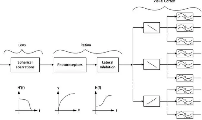
A block diagram of the HVS model is shown in Figure 2-3, where parts related to the lens, the retina, and the visual cortex, are indicated.
Figure 2-3. A block diagram of the HVS
In Figure 2-3, the first block is a spatial, isotropic, low-pass filter. It represents the spherical aberration of the lens, the effect of the pupil, and the frequency limitation by the finite number of photoreceptors. It is followed by the nonlinear characteristic of the photoreceptors, represented by a logarithmic curve. At the level of the retina, this nonlinear transformation is followed by an isotropic high-pass filter corresponding to the lateral inhibition phenomenon. Finally, there is a directional filter bank that represents the processing performed by the cells of the visual cortex. The bars in the boxes indicate the directional filters. This is followed by another filter bank, represented by the double waves, for detecting the intensity of the stimulus. It is worth mentioning that the overall system is shift-variant because of the decrease in resolution away from the fovea.8
Expoliting the HVS
By taking advantage of the characteristics of the HVS, and by tuning the parameters of the HVS model, tradeoffs can be made between visual quality loss and video data compression. In particular, the following benefits may be accrued.
By limiting the bandwidth, the visual signal may be sampled in •
spatial or temporal dimensions at a frequency equal to twice the bandwidth, satisfying the Nyquist criteria of sampling, without loss of visual quality.
The sensitivity of the HVS is decreased during rapid large-scale •
scene change and intense motion of objects, resulting in temporal or motion masking. In such cases the visibility thresholds are elevated due to temporal discontinuities in intensity. This can be exploited to achieve more efficient compression, without producing noticeable artifacts.
Texture information can be compressed more than motion •
information with negligible loss of visual quality. As discussed later in this chapter, several lossy compression algorithms allow quantization and resulting quality loss of texture information, while encoding the motion information losslessly.
Owing to low sensitivity of the HVS to the loss of color •
information, chroma subsampling is a feasible technique to reduce data rate without significantly impacting the visual quality.
Compression of brightness and contrast information can be •
achieved by discarding high-frequency information. This would impair the visual quality and introduce artifacts, but parameters of the amount of loss are controllable.
The HVS is sensitive to structural distortion. Therefore, measuring •
such distortions, especially for highly structured data such as image or video, would give a criterion to assess whether the amount of distortion is acceptable to human viewers. Although acceptability is subjective and not universal, structural distortion metrics can be used as an objective evaluation criterion.
The HVS allows humans to pay more attention to interesting parts •
An Overview of Compression Techniques
A high-definition uncompressed video data stream requires about 2 billion bits per second of data bandwidth. Owing to the large amount of data necessary to represent digital video, it is desirable that such video signals are easy to compress and decompress, to allow practical storage or transmission. The term data compression refers to the reduction in the number of bits required to store or convey data—including numeric, text, audio, speech, image, and video—by exploiting statistical properties of the data. Fortunately, video data is highly compressible owing to its strong vertical, horizontal, and temporal correlation and its redundancy.
Transform and prediction techniques can effectively exploit the available correlation, and information coding techniques can take advantage of the statistical structures present in video data. These techniques can be lossless, so that the reverse operation (decompression) reproduces an exact replica of the input. In addition, however, lossy techniques are commonly used in video data compression, exploiting the characteristics of the HVS, which is less sensitive to some color losses and some special types of noises.
Video compression and decompression are also known as video encoding and
decoding, respectively, as information coding principles are used in the compression and decompression processes, and the compressed data is presented in a coded bit stream format.
Data Structures and Concepts
Digital video signal is generally characterized as a form of computer data. Sensors of video signals usually output three color signals–red, green and blue (RGB)—that are individually converted to digital forms and are stored as arrays of picture elements (pixels), without the need of the blanking or sync pulses that were necessary for analog video signals. A two-dimensional array of these pixels, distributed horizontally and vertically, is called an image or a bitmap, and represents a frame of video. A time-dependent collection of frames represents the full video signal. There are five parameters9
associated with a bitmap: the starting address in memory, the number of pixels per line, the pitch value, the number of lines per frame, and the number of bits per pixel. In the following discussion, the terms frame and image are used interchangeably.
Signals and Sampling
The conversion of a continuous analog signal to a discrete digital signal, commonly known as the analog-to-digital (A/D) conversion, is done by taking samples of the analog signal at appropriate intervals in a process known as sampling. Thus x(n) is called the sampled version of the analog signal xa(t) if x(n) = xa(nT) for some T > 0, where T is known as the sampling period and 2π/T is known as the sampling frequency or the sampling rate. Figure 2-4 shows a spatial domain representation of xa(t) and corresponding x(n).
The frequency-domain representation of the signal is obtained by using the Fourier transform, which gives the analog frequency response Xa(jΩ) replicated at uniform intervals 2π/T, while the amplitudes are reduced by a factor of T. Figure 2-5 shows the concept.
Figure 2-4. Spatial domain representation of an analog signal and its sampled version
Figure 2-5. Fourier transform of a sampled analog bandlimited signal
If there is overlap between the shifted versions of Xa(jΩ), aliasing occurs because there are remnants of the neighboring copies in an extracted signal. However, when there is no aliasing, the signal xa(t) can be recovered from its sampled version x(n) by retaining only one copy.10 Thus if the signal is band-limited within a frequency band − π/T to π/T,
a sampling rate of 2π/T or more guarantees an alias-free sampled signal, where no actual information is lost due to sampling. This is called the Nyquist sampling rate, named after Harry Nyquist, who in 1928 proposed the above sampling theorem. Claude Shannon proved this theorem in 1949, so it is also popularly known as Nyquist-Shannon sampling theorem.
The theorem applies to single- and multi-dimensional signals. Obviously, compression of the signal can be achieved by using fewer samples, but in the case of sampling frequency less than twice the bandwidth of the signal, annoying aliasing artifacts will be visible.
10P.Vaidyanathan,MultirateSystemsandFilterBanks(EnglewoodCliffs:PrenticeHall
Common Terms and Notions
There are a few terms to know that are frequently used in digital video. The aspect ratio of a geometric shape is the ratio between its sizes in different dimensions. For example, the aspect ratio of an image is defined as the ratio of its width to its height. The display aspect ratio (DAR) is the width to height ratio of computer displays, where common ratios are 4:3 and 16:9 (widescreen). An aspect ratio for the pixels within an image is also defined. The most commonly used pixel aspect ratio (PAR) is 1:1 (square); other ratios, such as 12:11 or 16:11, are no longer popular. The term storage aspect ratio (SAR) is used to describe the relationship between the DAR and the PAR such that SAR × PAR = DAR.
Historically, the role of pixel aspect ratio in the video industry has been very important. As digital display technology, digital broadcast technology, and digital video compression technology evolved, using the pixel aspect ratio has been the most popular way to address the resulting video frame differences. However, today, all three technologies use square pixels predominantly.
As other colors can be obtained from a linear combination of primary colors such as red, green and blue in RGB color model, or cyan, magenta, yellow, and black in CMYK model, these colors represent the basic components of a color space spanning all colors. A complete subset of colors within a given color space is called a color gamut. Standard RGB (sRGB) is the most frequently used color space for computers. International Telecommunications Union (ITU) has recommended color primaries for standard definition (SD), high-definition (HD) and ultra-high-definition (UHD) televisions. These recommendations are included in internationally recognized digital studio standards defined by ITU-R recommendation BT.601,11 BT.709, and BT.2020, respectively. The sRGB
uses the ITU-R BT.709 color primaries.
Luma is the brightness of an image, and is also known as the black-and-white
information of the image. Although there are subtle differences between luminance
as used in color science and luma as used in video engineering, often in the video discussions these terms are used interchangeably. In fact, luminance refers to a linear combination of red, green, and blue color representing the intensity or power emitted per unit area of light, while luma refers to a nonlinear combination of R ’ G ’ B ’, the nonlinear function being known as the gamma function (y = xg, g = 0.45). The primes are used to
indicate nonlinearity. The gamma function is needed to compensate for properties of perceived vision, so as to perceptually evenly distribute the noise across the tone scale from black to white, and to use more bits to represent the color information that is more sensitive to human eyes. For details, see Poynton.12
Luma is often described along with chroma, which is the color information. As human vision has finer sensitivity to luma rather than chroma, chroma information is often subsampled without noticeable visual degradation, allowing lower resolution processing and storage of chroma. In component video, the three color components are
transmitted separately.13 Instead of sending R' G' B' directly, three derived components
are sent—namely the luma (Y') and two color difference signals (B' – Y') and (R' – Y'). While in analog video, these color difference signals are represented by U and V, respectively, in digital video, they are known as CB and CR components, respectively. In fact, U and V apply to analog video only, but are commonly, albeit inappropriately, used in digital video as well. The term chroma represents the color difference signals themselves; this term should not be confused with chromaticity, which represents the characteristics of the color signals.
In particular, chromaticity refers to an objective measure of the quality of color information only, not accounting for the luminance quality. Chromaticity is characterized by the hue and the saturation. The hue of a color signal is its “redness,” “greenness,” and so on. The hue is measured as degrees in a color wheel from a single hue. The saturation or colorfulness of a color signal is the degree of its difference from gray.
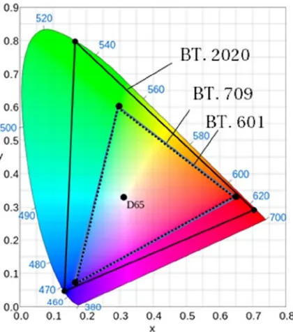
Figure 2-6 depicts the chromaticity diagram for the ITU-R recommendation BT.709 and BT.2020, showing the location of the red, green, blue, and white colors. Owing to the differences shown in this diagram, digital video signal represented in BT.2020 color primaries cannot be directly presented to a display that is designed according to BT.709; a conversion to the appropriate color primaries would be necessary in order to faithfully reproduce the actual colors.
Figure 2-6. ITU-R Recommendation BT.601, BT.709 and BT.2020 chromaticity diagram and location of primary colors. The point D65 shows the white point. (Courtesy of Wikipedia)
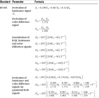
In order to convert R' G' B' samples to corresponding Y ' CBCR samples, in general, the following formulas are used:
Y K R K G K B
C B Y
K
C R Y
K
r g b
B
b
R
r
¢ ¢ ¢ ¢
¢ ¢
¢ ¢
= + +
=
-(
)
=
-(
)
2 1
2 1
(Eq. 2-1)
Each of the ITU-R recommendations mentioned previously uses the values of constants Kr, Kg , and Kb , as shown in Table 2-2, although the constant names are not defined as such in the specifications.
Table 2-2. Constants of R' G' B' Coefficients to Form Luma and Chroma Components
Standard
K
rK
gK
bBT.2020 0.2627 0.6780 0.0593
BT.709 0.2126 0.7152 0.0722
BT.601 0.2990 0.5870 0.1140
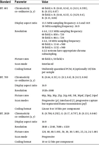
In addition to the signal formats, the recommendations also specify the opto-electronic conversion parameters and the picture characteristics. Table 2-4 shows some of these parameters.
Note: Here, Ek'is the original analog signal, D k
'is the coded digital signal, n is the number of
Table 2-4. Important Parameters in ITU-R Digital Video Studio Standards
Standard
Parameter
Value
BT. 601 Chromaticity co-ordinates (x, y)
60 field/s: R: (0.63, 0.34), G: (0.31, 0.595), B: (0.155, 0.07)
50 field/s: R: (0.64, 0.33), G: (0.29, 0.6), B: (0.15, 0.06)
Display aspect ratio 13.5 MHz sampling frequency: 4:3 and 16:9 18 MHz sampling frequency: 16:9
Resolution 4:4:4, 13.5 MHz sampling frequency: 60 field/s: 858 × 720
50 field/s: 864 × 720
4:4:4, 18 MHz sampling frequency: 60 field/s: 1144 × 960
50 field/s: 1152 × 960
4:2:2 systems have appropriate chroma subsampling.
Picture rates 60 field/s, 50 field/s
Scan mode Interlaced
Coding format Uniformly quantized PCM, 8 (optionally 10) bits per sample
BT. 709 Chromaticity co-ordinates (x, y)
R: (0.64, 0.33), G: (0.3, 0.6), B: (0.15, 0.06)
Display aspect ratio 16:9
Resolution 1920×1080
Picture rates 60p, 50p, 30p, 25p, 24p, 60i, 50i, 30psf, 25psf, 24psf
Scan modes Progressive (p), interlaced (i), progressive capture but segmented frame transmission (psf)
Coding format Linear 8 or 10 bits per component
BT. 2020 Chromaticity co-ordinates (x, y)
R: (0.708, 0.292), G: (0.17, 0.797), B: (0.131, 0.046)
Display aspect ratio 16:9
Resolution 3840 × 2160, 7680 × 4320
Picture rates 120, 60, 60/1.001, 50, 30, 30/1.001, 25, 24, 24/1.001
Scan mode Progressive
Chroma Subsampling
As mentioned earlier, the HVS is less sensitive to color information compared to its sensitivity to brightness information. Taking advantage of this fact, technicians developed methods to reduce the chroma information without significant loss in visual quality. Chroma subsampling is a common data-rate reduction technique and is used in both analog and digital video encoding schemes. Besides video, it is also used, for example, in popular single-image coding algorithms, as defined by the Joint Photographic Experts Group (JPEG), a joint committee between the International Standards Organization (ISO) and the ITU-T.
Exploiting the high correlation in color information and the characteristics of the HVS, chroma subsampling reduces the overall data bandwidth. For example, a 2:1 chroma subsampling of a rectangular image in the horizontal direction results in only two-thirds of the bandwidth required for the image with full color resolution. However, such saving in data bandwidth is achieved with little perceptible visual quality loss at normal viewing distances.
4:4:4 to 4:2:0
Typically, images are captured in the R ' G ' B ' color space, and are converted to the
Y ' UV color space (or for digital video Y 'CBCR; in the discussion we use Y ' UV and Y 'CBCR
interchangeably for simplicity) using the conversion matrices described earlier. The resulting Y 'UV image is a full-resolution image with a 4:4:4 sampling ratio of the Y ', U and
V components, respectively. This means that for every four samples of Y ' (luma), there are four samples of U and four samples of V chroma information present in the image.
The ratios are usually defined for a 4×2 sample region, for which there are four 4×2 luma samples. In the ratio 4 : a : b, a and b are determined based on the number of chroma samples in the top and bottom row of the 4 × 2 sample region. Accordingly, a 4:4:4 image has full horizontal and vertical chroma resolution, a 4:2:2 image has a half-horizontal and full vertical resolution, and a 4:2:0 image has half resolutions in both horizontal and vertical dimensions.
A subsampling is also known as downsampling, or sampling rate compression. If the input signal is not bandlimited in a certain way, subsampling results in aliasing and information loss, and the operation is not reversible. To avoid aliasing, a low pass filter is used before subsampling in most appplications, thus ensuring the signal to be bandlimited.
The 4:2:0 images are used in most international standards, as this format provides sufficient color resolution for an acceptable perceptual quality, exploiting the high correlation between color components. Therefore, often a camera-captured R'G'B' image is converted to Y 'UV 4:2:0 format for compression and processing. In order to convert a 4:4:4 image to a 4:2:0 image, typically a two-step approach is taken. First, the 4:4:4 image is converted to a 4:2:2 image via filtering and subsampling horizontally; then, the resulting image is converted to a 4:2:0 format via vertical filtering and subsampling. Example filters are shown in Figure 2-8.
Figure 2-8. Typical symmetric finite impulse response (FIR) filters used for 2:1 subsampling
Table 2-5. FIR Filter Coefficients of a 2:1 Horizontal and a 2:1 Vertical Filter, Typically Used in 4:4:4 to 4:2:0 Conversion
Filter Coefficients
Horiz. 0.0430 0.0000 -0.1016 0.0000 0.3105 0.5000 0.3105 0.0000 -0.1016 0.0000 0.0430
Vert. 0.0098 0.0215 -0.0410 -0.0723 0.1367 0.4453 0.1367 -0.0723 -0.0410 0.0215 0.0098
Norm. Freq.
-0.5 -0.4 -0.3 -0.2 -0.1 0 0.1 0.2 0.3 0.4 0.5 The filter coefficients for the Figure 2-8 finite impulse response (FIR) filters are given in Table 2-5. In this example, while the horizontal filter has zero phase difference, the vertical filter has a phase shift of 0.5 sample interval.
Reduction of Redundancy
Spatial Redundancy
The digitization process ends up using a large number of bits to represent an image or a video frame. However, the number of bits necessary to represent the information content of a frame may be substantially less, due to redundancy. Redundancy is defined as 1 minus the ratio of the minimum number of bits needed to represent an image to the actual number of bits used to represent it. This typically ranges from 46 percent for images with a lot of spatial details, such as a scene of foliage, to 74 percent14 for low-detail
images, such as a picture of a face. Compression techniques aim to reduce the number of bits required to represent a frame by removing or reducing the available redundancy.
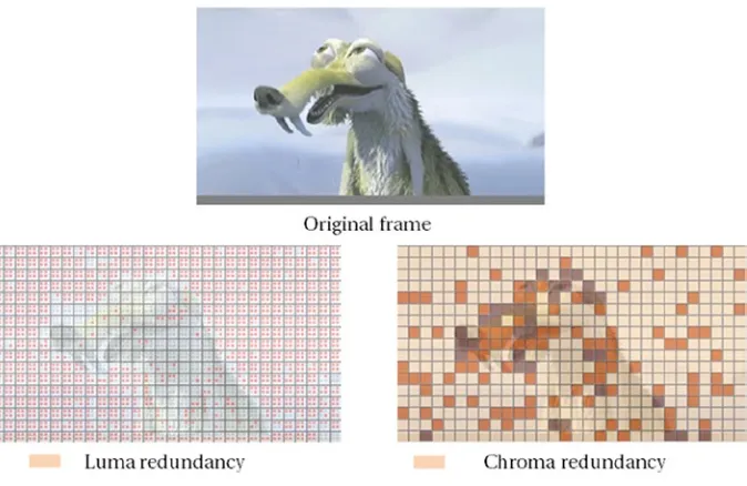
Spatial redundancy is the consequence of the correlation in horizontal and the vertical spatial dimensions between neighboring pixel values within the same picture or frame of video (also known as intra-picture correlation). Neighboring pixels in a video frame are often very similar to each other, especially when the frame is divided into the luma and the chroma components. A frame can be divided into smaller blocks of pixels to take advantage of such pixel correlations, as the correlation is usually high within a block. In other words, within a small area of the frame, the rate of change in a spatial dimension is usually low. This implies that, in a frequency-domain representation of the video frame, most of the energy is often concentrated in the low-frequency region, and high-frequency edges are relatively rare. Figure 2-9 shows an example of spatial redundancy present in a video frame.
Figure 2-9. An example of spatial redundancy in an image or a video frame
14M.RabbaniandP.Jones,DigitalImageCompressionTechniques(Bellingham,WA:SPIEOptical
The redundancy present in a frame depends on several parameters. For example, the sampling rate, the number of quantization levels, and the presence of source or sensor noise can all affect the achievable compression. Higher sampling rates, low quantization levels, and low noise mean higher pixel-to-pixel correlation and higher exploitable spatial redundancy.
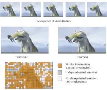
Temporal Redundancy
Temporal redundancy is due to the correlation between different pictures or frames in a video (also known as inter-picture correlation). There is a significant amount of temporal redundancy present in digital videos. A video is frequently shown at a frame rate of more than 15 frames per second (fps) in order for a human observer to perceive a smooth, continuous motion; this requires neighboring frames to be very similar to each other. One such example is shown in Figure 2-10. It may be noted that a reduced frame rate would result in data compression, but that would be at the expense of perceptible
flickering artifact.
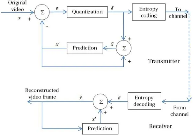
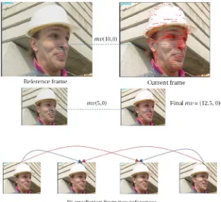
Thus, a frame can be represented in terms of a neighboring reference frame and the difference information between these frames. Because an independent frame is reconstructed at the receiving end of a transmission system, it is not necessary for a dependent frame to be transmitted. Only the difference information is sufficient for the successful reconstruction of a dependent frame using a prediction from an already received reference frame. Due to temporal redundancy, such difference signals are often quite small. Only the difference signal can be coded and sent to the receiving end, while the receiver can combine the difference signal with the predicted signal already available and obtain a frame of video, thereby achieving very high amount of compression. Figure 2-11 shows an example of how temporal redundancy is exploited.
Figure 2-12. An example of reduction of informataion via motion compensation
Figure 2-11. Prediction and reconstruction process exploiting temporal redundancy
The prediction and reconstruction process is lossless. However, it is easy to understand that the better the prediction, the less information remains in the difference signal, resulting in a higher compression. Therefore, every new generation of international video coding standards has attempted to improve upon the prediction process of the previous generation.
Statistical Redundancy
In information theory, redundancy is the number of bits used to transmit a signal minus the number of bits of actual information in the signal, normalized to the number of bits used to transmit the signal. The goal of data compression is to reduce or eliminate unwanted redundancy. Video signals characteristically have various types of redundancies, including spatial and temporal redundancies, as discussed above. In addition, video signals contain statistical redundancy in its digital representation; that is, there are usually extra bits that can be eliminated before transmission.
For example, a region in a binary image (e.g., a fax image or a video frame) can be viewed as a string of 0s and 1s, the 0s representing the white pixels and 1s representing the black pixels. These strings, where the same bit occurs in a series or run of consecutive data elements, can be represented using run-length codes; these codes the address of each string of 1s (or 0s) followed by the length of that string. For example, 1110 0000 0000 0000 0000 0011 can be coded using three codes (1,3), (0,19), and (1,2), representing 3 1s, 19 0s, and 2 1s. Assuming only two symbols, 0 and 1, are present, the string can also be coded using two codes (0,3) and (22,2), representing the length of 1s at locations 0 and 22.
Variations on the run-length are also possible. The idea is this: instead of the original data elements, only the number of consecutive data elements is coded and stored, thereby achieving significant data compression. Run-length coding is a lossless data compression technique and is effectively used in compressing quantized coefficients, which contains runs of 0s and 1s, especially after discarding high-frequency information.
According to Shannon’s source coding theorem, the maximum achievable compression by exploiting statistical redundancy is given as:
C average bit rate of the original signal B average bit
= ( )
rrate of the encoded data H( )
Here, H is the entropy of the source signal in bits per symbol. Although this theoretical limit is achievable by designing a coding scheme, such as vector quantization
or block coding, for practical video frames—for instance, video frames of size 1920 × 1080 pixels with 24 bits per pixel—the codebook size can be prohibitively large.15 Therefore,
international standards instead often use entropy coding methods to get arbitrarily close to the theoretical limit.
15A.K.Jain,FundamentalsofDigitalImageProcessing(EnglewoodCliffs:Prentice-Hall
Entropy Coding
Consider a set of quantized coefficients that can be represented using B bits per pixel. If the quantized coefficients are not uniformly distributed, then their entropy will be less than B bits per pixel. Now, consider a block of M pixels. Given that each bit can be one of two values, we have a total number of L = 2MB different pixel blocks.
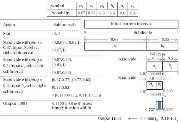
For a given set of data, let us assign the probability of a particular block i occurring as pi, where i = 0, 1, 2, ···, L − 1. Entropy coding is a lossless coding scheme, where the goal is to encode this pixel block using − log2pi bits, so that the average bit rate is equal to the entropy of the M pixel block: H = ∑ ipi(−log2pi). This gives a variable length code for each block of M pixels, with smaller code lengths assigned to highly probable pixel blocks. In most video-coding algorithms, quantized coefficients are usually run-length coded, while the resulting data undergo entropy coding for further reduction of statistical redundancy.
For a given block size, a technique called Huffman coding is the most efficient and popular variable-length encoding method, which asymptotically approaches Shannon’s limit of maximum achievable compression. Other notable and popular entropy coding techniques are arithmetic coding and Golomb-Rice coding.
Golomb-Rice coding is especially useful when the approximate entropy
characteristics are known—for example, when small values occur more frequently than large values in the input stream. Using sample-to-sample prediction, the Golomb-Rice coding scheme produces output rates within 0.25 bits per pixel of the one-dimensional difference entropy for entropy values ranging from 0 to 8 bits per pixel, without needing to store any code words. Golomb-Rice coding is essentially an optimal run-length code. To compare, we discuss now the Huffman coding and the arithmetic coding.
Huffman Coding
Huffman coding is the most popular lossless entropy coding algorithm; it was developed by David Huffman in 1952. It uses a variable-length code table to encode a source symbol, while the table is derived based on the estimated probability of occurrence for each possible value of the source symbol. Huffman coding represents each source symbol in such a way that the most frequent source symbol is assigned the shortest code and the least frequent source symbol is assigned the longest code. It results in a prefix code, so that a bit string representing a source symbol is never a prefix of the bit string representing another source symbol, thereby making it uniquely decodable.
To understand how Huffman coding works, let us consider a set of four source symbols {a0, a1, a2, a3} with probabilities {0.47, 0.29, 0.23, 0.01}, respectively. First, a binary tree is generated from left to right, taking the two least probable symbols and combining them into a new equivalent symbol with a probability equal to the sum of the probablities of the two symbols. In our example, therefore, we take a2 and a3 and form a new symbol
b2 with a probability 0.23 + 0.01 = 0.24. The process is repeated until there is only one symbol left.
1 for c1. This codeword is the prefix for all its branches, ensuring unique decodeability. At the next branch level, codeword 10 (two bits) is assigned to the next probable symbol
a1, while 11 goes to b2 and as a prefix to its branches. Thus, a2 and a3 receive codewords 110 and 111 (three bits each), respectively. Figure 2-13 shows the process and the final Huffman codes.
Figure 2-13. Huffman coding example
While these four symbols could have been assigned fixed length codes of 00, 01, 10, and 11 using two bits per symbol, given that the probability distribution is non-uniform and the entropy of these symbols is only 1.584 bits per symbol, there is room for improvement. If these codes are used, 1.77 bits per symbol will be needed instead of two bits per symbol. Although this is still 0.186 bits per symbol apart from the theoretical minimum of 1.584 bits per symbol, it still provides approximately 12 percent compression compared to fixed-length code. In general, the larger the difference in probabilities between the most and the least probable symbols, the larger the coding gain Huffman coding would provide. Huffman coding is optimal when the probability of each input symbol is the inverse of a power of 2.