Edward A. Lee and Pravin Varaiya
[email protected], [email protected] Electrical Engineering & Computer Science
University of California, Berkeley
Copyright c2000
Preface xiii
Notes to Instructors xvii
1 Signals and Systems 1
1.1 Signals. . . 2
1.1.1 Audio signals . . . 2
1.1.2 Images . . . 5
Probing further: Household electrical power . . . 7
1.1.3 Video signals . . . 10
1.1.4 Signals representing physical attributes . . . 12
1.1.5 Sequences. . . 13
1.1.6 Discrete signals and sampling . . . 14
1.2 Systems . . . 19
1.2.1 Systems as functions . . . 19
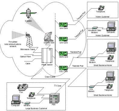
1.2.2 Telecommunications systems. . . 20
Probing further: Wireless communication . . . 23
Probing further: LEO telephony . . . 24
Probing further: Encrypted speech . . . 28
1.2.3 Audio storage and retrieval. . . 29
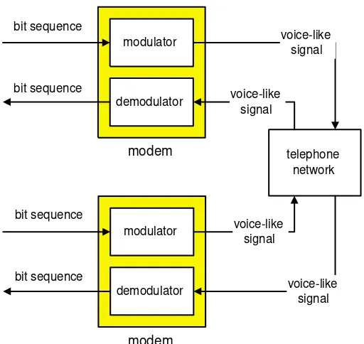
1.2.4 Modem negotiation. . . 30
1.2.5 Feedback control system . . . 31
1.3 Summary . . . 34
2 Defining Signals and Systems 37
2.1 Defining functions . . . 37
2.1.1 Declarative assignment . . . 37
2.1.2 Graphs . . . 39
Probing further: Relations . . . 41
2.1.3 Tables . . . 41
2.1.4 Procedures . . . 42
2.1.5 Composition . . . 42
Probing further: Declarative interpretation of imperative definitions . . . 46
2.1.6 Declarative vs. imperative . . . 47
2.2 Defining signals . . . 48
2.2.1 Declarative definitions . . . 49
2.2.2 Imperative definitions . . . 49
2.2.3 Physical modeling . . . 50
Probing further: Physics of a Tuning Fork . . . 51
2.3 Defining systems . . . 52
2.3.1 Memoryless systems . . . 53
2.3.2 Differential equations. . . 53
2.3.3 Difference equations . . . 54
2.3.4 Composing systems using block diagrams. . . 56
Probing further: Composition of graphs . . . 58
3 State-Space Models 65 3.1 State machines . . . 65
3.1.1 Updates . . . 67
3.1.2 Stuttering . . . 67
3.2 Finite state machines . . . 69
3.2.1 State transition diagrams . . . 69
3.2.2 Update table . . . 74
3.4 Simulation and bisimulation . . . 83
3.4.1 Relating behaviors . . . 88
4 Composing State Machines 97 4.1 Synchrony . . . 97
4.2 Side-by-side composition . . . 98
4.3 Cascade composition . . . 100
4.4 Product-form inputs and outputs . . . 104
4.5 General feedforward composition . . . 106
4.6 Hierarchical composition . . . 108
4.7 Feedback . . . 110
4.7.1 Feedback composition with no inputs . . . 111
4.7.2 Feedback composition with inputs . . . 116
Probing further: Least fixed point. . . 117
4.7.3 Feedback composition of multiple machines. . . 118
4.8 Nondeterministic machines . . . 122
5 Linear Systems 127 5.1 Operation of an infinite state machine . . . 128
Basics: Arithmetic on tuples of real numbers. . . 129
5.1.1 Time . . . 129
Basics: Functions yielding tuples. . . 130
Basics: Linear functions . . . 132
5.2 One-dimensional SISO systems . . . 133
5.2.1 Zero-state and zero-input response. . . 136
Basics: Matrices and vectors . . . 138
Basics: Matrix arithmetic . . . 139
5.4 Multidimensional MIMO systems . . . 143
5.5 Linear systems . . . 144
5.6 Continuous-time state-space models . . . 144
Probing further: Approximating continuous-time systems. . . 145
6 Frequency Domain 149 6.1 Frequency decomposition. . . 150
Basics: Frequencies in Hertz and radians. . . 151
Basics: Ranges of frequencies . . . 152
Probing further: Circle of fifths. . . 154
6.2 Phase . . . 155
6.3 Spatial frequency . . . 156
6.4 Periodic and finite signals. . . 157
6.5 Fourier series . . . 158
Probing further: Convergence of the Fourier series. . . 164
6.5.1 Uniqueness of the Fourier series . . . 165
6.5.2 Periodic, finite, and aperiodic signals . . . 165
6.5.3 Fourier series approximations to images. . . 167
6.6 Discrete-time signals . . . 167
Basics: Discrete-time frequencies . . . 168
6.6.1 Periodicity . . . 168
6.6.2 The discrete-time Fourier series . . . 169
Exercises . . . 170
7 Frequency Response 175 7.1 LTI systems . . . 176
7.1.1 Time invariance. . . 176
7.1.2 Linearity . . . 178
7.1.3 Linearity and time-invariance . . . 180
Tips and Tricks: Phasors . . . 185
7.2.1 The Fourier series with complex exponentials . . . 190
7.2.2 Examples . . . 191
7.3 Determining the Fourier series coefficients. . . 191
Probing further: Relating DFS coefficients . . . 192
Probing further: Formula for Fourier series coefficients . . . 194
Probing further: Exchanging integrals and summations . . . 195
7.3.1 Negative frequencies . . . 195
7.4 Frequency response and the fourier series . . . 195
7.5 Frequency response of composite systems . . . 196
7.5.1 Cascade connection. . . 196
7.5.2 Feedback connection . . . 198
Probing further: Feedback systems are LTI. . . 200
8 Filtering 205 8.1 Convolution . . . 206
8.1.1 Convolution sum and integral . . . 208
8.1.2 Impulses . . . 211
8.1.3 Signals as sums of weighted delta functions . . . 212
8.1.4 Impulse response and convolution . . . 214
8.2 Frequency response and impulse response . . . 217
8.3 Causality . . . 220
8.4 Finite impulse response (FIR) filters . . . 220
Probing further: Causality . . . 221
8.4.1 Design of FIR filters . . . 223
8.4.2 Decibels. . . 227
Probing further: Decibels . . . 229
8.5.1 Designing IIR filters . . . 230
8.6 Implementation of filters . . . 232
8.6.1 Matlab implementation. . . 234
8.6.2 Signal flow graphs . . . 234
Probing further: Java implementation of an FIR filter . . . 235
Probing further: Programmable DSP implementation of an FIR filter . . . 236
9 The Four Fourier Transforms 245 9.1 Notation . . . 245
9.2 The Fourier series (FS) . . . 246
9.3 The discrete Fourier transform (DFT) . . . 247
Probing further: Showing inverse relations . . . 248
9.4 The discrete-Time Fourier transform (DTFT) . . . 250
9.5 The continuous-time Fourier transform. . . 251
Probing further: Multiplying signals . . . 253
9.6 Relationship to convolution. . . 254
9.7 Properties and examples . . . 254
9.7.1 Conjugate symmetry . . . 254
9.7.2 Time shifting . . . 255
9.7.3 Linearity . . . 258
9.7.4 Constant signals . . . 259
9.7.5 Frequency shifting and modulation . . . 260
10 Sampling and Reconstruction 267 10.1 Sampling . . . 267
Basics: Units . . . 268
10.1.1 Sampling a sinusoid . . . 268
10.1.2 Aliasing . . . 268
10.1.3 Perceived pitch experiment. . . 270
10.3 The Nyquist-Shannon sampling theorem . . . 277
Probing further: Sampling . . . 278
A Sets and Functions 285 A.1 Sets . . . 285
A.1.1 Assignment and assertion . . . 286
A.1.2 Sets of sets . . . 287
A.1.3 Variables and predicates . . . 287
Probing further: Predicates in Matlab. . . 288
A.1.4 Quantification over sets. . . 289
A.1.5 Some useful sets . . . 290
A.1.6 Set operations: union, intersection, complement. . . 291
A.1.7 Predicate operations . . . 291
A.1.8 Permutations and combinations . . . 293
A.1.9 Product sets . . . 293
Basics: Tuples, strings, and sequences . . . 294
A.1.10 Evaluating a predicate expression . . . 299
A.2 Functions . . . 302
A.2.1 Defining functions . . . 303
A.2.2 Tuples and sequences as functions . . . 304
A.2.3 Function properties . . . 304
Probing further: Infinite sets . . . 305
Probing further: Even bigger sets. . . 306
A.3 Summary . . . 307
B Complex Numbers 311 B.1 Imaginary numbers . . . 311
B.3 Complex numbers . . . 313
B.4 Arithmetic of complex numbers . . . 314
B.5 Exponentials . . . 315
B.6 Polar coordinates . . . 316
C Laboratory Exercises 323 C.1 Arrays and sound . . . 326
C.1.1 In-lab section . . . 326
C.1.2 Independent section . . . 329
C.2 Images. . . 332
C.2.1 Images in Matlab . . . 332
C.2.2 In-lab section . . . 334
C.2.3 Independent section . . . 336
C.3 State machines . . . 340
C.3.1 Background . . . 340
C.3.2 In-lab section . . . 343
C.3.3 Independent section . . . 344
C.4 Control systems . . . 347
C.4.1 Background . . . 347
C.4.2 In-lab section . . . 349
C.4.3 Independent section . . . 350
C.5 Difference equations . . . 352
C.5.1 In-lab section . . . 352
C.5.2 Independent section . . . 353
C.6 Differential equations . . . 356
C.6.1 Background . . . 356
C.6.2 In-lab section . . . 358
C.6.3 Independent section . . . 359
C.7 Spectrum . . . 363
C.8 Comb filters . . . 372
C.8.1 Background . . . 372
C.8.2 In-lab section . . . 375
C.8.3 Independent section . . . 376
C.9 Plucked string instrument . . . 378
C.9.1 Background . . . 378
C.9.2 In-lab section . . . 380
C.9.3 Independent section . . . 381
C.10 Modulation and demodulation . . . 384
C.10.1 Background . . . 384
C.10.2 In-lab section . . . 390
C.10.3 Independent section . . . 391
C.11 Sampling and aliasing. . . 393
C.11.1 In-lab section . . . 393
This book is a reaction to a trauma in our discipline. We have all been aware for some time that “electrical engineering” has lost touch with the “electrical.” Electricity provides the impetus, the pressure, thepotential, but not the body. How else could microelectromechanical systems (MEMS) become so important in EE? Is this not a mechanical engineering discipline? Or signal processing. Is this not mathematics? Or digital networking. Is this not computer science? How is it that control system are applied equally comfortably to aeronautical systems, structural mechanics, electrical systems, and options pricing?
Like so many engineering schools, Berkeley used to have an introductory course entitled “Intro-duction to Electrical Engineering” that was about analog circuits. This quaint artifact spoke more about the origins of the discipline that its contemporary reality. Like engineering topics in schools of mining (which Berkeley’s engineering school once was), ours has evolved more rapidly than the institutional structure around it.
Abelson and Sussman, inStructure and Interpretation of Computer Programs(MIT Press), a book that revolutionized computer science education, faced a similar transition in their discipline.
“Underlying our approach to this subject is our conviction that ‘computer science’ is not a science and that its significance has little to do with computers.”
Circuits used to be the heart of electrical engineering. It is arguable that today it is the analytical techniques that emerged from circuit theory that are the heart of the discipline. The circuits them-selves have become an area of specialization. It is an important area of specialization, to be sure, with high demand for students, who command high salaries. But it is a specialization nonetheless.
Before Abelson and Sussman, computer programming was about getting computers to do your bidding. In the preface toStructure and Interpretation of Computer Programs, they say
“First, we want to establish the idea that a computer language is not just a way of getting a computer to perform operations but rather that it is a novel formal medium for expressing ideas about methodology. Thus, programs must be written for people to read, and only incidentally for machines to execute.”
In the origins of our discipline, a signal was a voltage that varies over time, an electromagnetic waveform, or an acoustic waveform. Now it is likely to be a sequence of discrete messages sent
over the internet using TCP/IP. Thestateof a system used to be adequately captured by variables in a differential equation. Now it is likely to be the registers and memory of a computer, or more abstractly, a process continuation, or a set of concurrent finite state machines. Asystem used to be well-modeled by a linear time-invariant transfer function. Now it is likely to be a computation in a Turing-complete computational engine. Despite these fundamental changes in the medium with which we operate, the methodology remains robust and powerful. It is the methodology, not the medium, that defines our field. Our graduates are more likely to write software than to push electrons, and yet we recognize them as electrical engineers.
Fundamental limits have also changed. Although we still face thermal noise and the speed of light, we are likely to encounter other limits before we get to these, such as complexity, computability, chaos, and, most commonly, limits imposed by other human constructions. A voiceband data mo-dem, for example, faces the telephone network, which was designed to carry voice, and offers as immutable limits such non-physical constraints as its 3 kHz bandwidth. DSL modems face reg-ulatory constraints that are more limiting than their physical constraints. Computer-based audio systems face latency and jitter imposed by the operating system.
The mathematical basis for the discipline has also shifted. Although we still use calculus and differential equations, we frequently need discrete math, set theory, and mathematical logic. Indeed, a major theme of this book is to illustrate that formal techniques can be used in a very wide range of contexts. Whereas the mathematics of calculus and differential equations evolved to describe the physical world, the world we face as system designers often has non-physical properties that are not such a good match to this mathematics. Instead of abandoning formality, we need to broaden the mathematical base.
Again, Abelson and Sussman faced a similar conundrum.
“... we believe that the essential material to be addressed by a subject at this level is not the syntax of particular programming language constructs, nor clever algorithms for computing particular functions efficiently, nor even the mathematical analysis of algorithms and the foundations of computing, but rather the techniques used to control the intellectual complexity of large software systems.”
This book is about signals and systems, not about large software systems. But it takes a compu-tational view of signals and systems. It focuses on the methods “used to control the intellectual complexity,” rather than on the physical limitations imposed by the implementations of old. Appro-priately, it puts emphasis on discrete-time modeling, which is pertinent to the implementations in software and digital logic that are so common today. Continuous-time models describe the physical world, with which our systems interact. But fewer of the systems we engineer operate directly in this domain.
temology– the study of the structure of knowledge from an imperative point of view, as opposed to the more declarative point of view taken by classical mathematical sub-jects. Mathematics provides a framework for dealing precisely with notions of ‘what is.’ Computation provides a fram-work for dealing precisely with notions of ‘how to’.”
Indeed, a major theme in our book is the connection between imperative (computational) and declar-ative (mathematical) descriptions of signals and systems. The laboratory component of the text, in our view, is an essential part of a complete study. The web content, with its extensive applets il-lustrating computational concepts, is an essential complement to the mathematics. Traditional elec-trical engineering has emphasized the declarative view. Modern elecelec-trical engineering has much closer ties to computer science, and has to complement this declarative view with an imperative one.
Besides being a proper part of the intellectual discipline, an imperative view has another key advan-tage. It enables a much closer connection with “real signals and systems,” which are often too messy for a complete declarative treatment. While a declarative treatment can easily handle a sinusoidal signal, an imperative treatment can easily handle a voice signal. One of our objectives in designing this text and the course on which it is based is to illustrate concepts with real signals and systemsat every step.
The course begins by describing signals as functions, focusing on characterizing the domain and the range. Systems are also described as functions, but now the domain and range are sets of signals. Characterizing these functions is thetopic of this course. Sets and functions provide the unifying notation and formalism.
We begin by describing systems using the notion of state, first using automata theory and then progressing to linear systems. Frequency domain concepts are introduced as a complementary toolset, different from that of state machines, and much more powerful when applicable. Frequency decomposition of signals is introduced using psychoacoustics, and gradually developed until all four Fourier transforms (the Fourier series, the Fourier transform, the discrete-time Fourier transform, and the DFT) have been described. We linger on the first of these, the Fourier series, since it is conceptually the easiest, and then quickly present the others as simple generalizations of the Fourier series. Finally, the course closes by using these concepts to study sampling and aliasing, which helps bridge the computational world with the physical world.
This text has evolved to support a course we now teach regularly at Berkeley to about 500 students per year. An extensive accompanying web page is organized around Berkeley’s 15 week semester, although we believe it can be adapted to other formats. The course organization at Berkeley is as follows:
Week 1 – Signals as Functions – Chapters 1 and 2.The first week motivates forthcoming material by illustrating how signals can be modeled abstractly as functions on sets. The emphasis is on characterizing the domain and the range, not on characterizing the function itself. The startup sequence of a voiceband data modem is used as an illustration, with a supporting applet that plays the very familiar sound of the startup handshake of V32.bis modem, and examines the waveform in both the time and frequency domain. The domain and range of the following signal types is given: sound, images, position in space, angles of a robot arm, binary sequences, word sequences, and event sequences.
Week 2 – Systems as Functions – Chapters 1 and 2. The second week introduces systems as functions that map functions (signals) into functions (signals). Again, it focuses not on how the function is defined, but rather on what is its domain and range. Block diagrams are defined as a visual syntax for composing functions. Applications considered are DTMF signaling, modems, digital voice, and audio storage and retrieval. These all share the property that systems are required to convert domains of functions. For example, to transmit a digital signal through the telephone system, the digital signal has to be converted into a signal in the domain of the telephone system
(i.e., a bandlimited audio signal).
Week 3 – State – Chapter 3.Week 3 is when the students start seriously the laboratory component of the course. The first lecture in this week is therefore devoted to the problem of relating declar-ative and imperdeclar-ative descriptions of signals and systems. This sets the framework for making the intellectual connection between the labs and the mathematics.
The purpose of this first lab exercise is to explore arrays in Matlab and to use them to construct audio signals. The lab is designed to help students become familiar with the fundamentals of Matlab, while applying it to synthesis of sound. In particular, it introduces the vectorization feature of the Matlab programming language. The lab consists of explorations with sinusoidal sounds with exponential envelopes, relating musical notes with frequency, and introducing the use of discrete-time (sampled) representations of continuous-time signals (sound).
Note that there is some potential confusion because Matlab uses the term “function” somewhat more loosely than the course does when referring to mathematical functions. Any Matlab command that takes arguments in parentheses is called a function. And most have a well-defined domain and range, and do, in fact, define a mapping from the domain to the range. These can be viewed formally as a (mathematical) functions. Some, however, such asplotandsoundare a bit harder to view this way. The last exercise in the lab explores this relationship.
The rest of the lecture content in the third week is devoted to introducing the notion of state and state machines. State machines are described by a functionupdatethat, given the current state and input, returns the new state and output. In anticipation of composing state machines, the concept of stutteringis introduced. This is a slightly difficult concept to introduce at this time because it has no utility until you compose state machines. But introducing it now means that we don’t have to change the rules later when we compose machines.
Week 4 – Nondeterminism and Equivalence – Chapter 3. The fourth week deals with nonde-terminism and equivalence in state machines. Equivalence is based on the notion of simulation, so simulation relations and bisimulation are defined for both deterministic and nondeterministic ma-chines. These are used to explain that two state machines may be equivalent even if they have a different number of states, and that one state machine may be an abstraction of another, in that it has all input/output behaviors of the other (and then some).
The most useful concept to help subsequent material is that feedback loops with delays are always well formed.
The lab in this week (C.3) uses Matlab as a low-level programming language to construct state machines according to a systematic design pattern that will allow for easy composition. The theme of the lab is establishing the correspondence between pictorial representations of finite automata, mathematical functions giving the state update, and software realizations.
The main project in this lab exercise is to construct a virtual pet. This problem is inspired by the Tamagotchi virtual pet made by Bandai in Japan. Tamagotchi pets, which translate as “cute little eggs,” were extremely popular in the late 1990’s, and had behavior considerably more complex than that described in this exercise. The pet is cat that behaves as follows:
It starts outhappy. If you petit, itpurrs. If youfeed it, itthrows up. Iftime passes, it getshungry andrubsagainst your legs. If you feed it when it is hungry, it purrs and gets happy. If you pet it when it is hungry, itbitesyou. If time passes when it is hungry, itdies.
The italicized words and phrases in this description should be elements in either the state space or the input or output alphabets. Students define the input and output alphabets and give a state transition diagram. They construct a function in Matlab that returns the next state and the output given the current state and the input. They then write a program to execute the state machine until the user types ’quit’ or ’exit.’
Next, the students design an open-loop controller that keeps the virtual pet alive. This illustrates that systematically constructed state machines can be easily composed.
This lab builds on the flow control constructs (for loops) introduced in the previous labs and intro-duces string manipulation and the use of M files.
Week 6 – Linear Systems.We consider linear systems as state machines where the state is a vector of reals. Difference equations and differential equations are shown to describe such state machines. The notions of linearity and superposition are introduced.
In the previous lab, students were able to construct an open-loop controller that would keep their virtual pet alive. In this lab (C.4), they modify the pet so that its behavior is nondeterministic. In particular, they modify the cat’s behavior so that if it is hungry and they feed it, it sometimes gets happy and purrs (as it did before), but it sometimes stays hungry and rubs against your legs. They then attempt to construct an open-loop controller that keeps the pet alive, but of course no such controller is possible without some feedback information. So they are asked to construct a state machine that can be composed in a feedback arrangement such that it keeps the cat alive.
of synchronous feedback.
In particular, the controller composed with the virtual pet does not, at first, seem to have enough information available to start the model executing. The input to the controller, which is the output of the pet, is not available until the input to the pet, which is the output of the controller, is available. There is a bootstrapping problem. The (better) students learn to design state machines that can resolve this apparent paradox.
Most students find this lab quite challenging, but also very gratifying when they figure it out. The concepts behind it are deep, and the better students realize that. The weaker students, however, just get by, getting something working without really understanding how to do it systematically.
Week 7 – Response of Linear Systems. Matrices and vectors are used to compactly describe systems with linear and time-invariant state updates. Impulses and impulse response are introduced. The deep concept here is linearity, and the benefits it brings, specifically being able to write the state and output response as a convolution sum.
We begin to develop frequency domain concepts, using musical notes as a way to introduce the idea that signals can be given as sums of sinusoids.
There is no lab exercise this week, giving students more time to prepare for the first midterm exam.
Week 8 – Frequency Domain. This week introduces frequency domain concepts and the Fourier series. Periodic signals are defined, and Fourier series coefficients are calculated by inspection for certain signals. The frequency domain decomposition is motivated by the linearity of systems considered last week (using the superposition principle), and by psychoacoustics and music.
In the lab in this week (C.5), the students build on the previous exercise by constructing state ma-chine models (now with infinite states and linear update equations). They build stable, unstable, and marginally stable state machines, describing them as difference equations.
The prime example of a stable system yields a sinusoidal signal with a decaying exponential enve-lope. The corresponding state machine is a simple approximate model of the physics of a plucked string instrument, such as a guitar. It is also the same signal that the students generated in the first lab by more direct (and more costly) methods. They compare the complexity of the state machine model with that of the sound generators that they constructed in the first lab, finding that the state machine model yields sinusoidal outputs with considerably fewer multiplies and adds than direct calculation of trigonometric and exponential functions.
The prime example of a marginally stable system is an oscillator. The students discover that an oscillator is just a boundary case between stable and unstable systems.
Week 9 – Frequency Response.In this week, we consider linear, time-invariant (LTI) systems, and introduce the notion of frequency response. We show that a complex exponential is an eigenfunction of an LTI system. The Fourier series is redone using complex exponentials, and frequency response is defined in terms of this Fourier series, for periodic inputs.
However, these are not as good for Simulink as for Matlab. The lab exercise have to guide the students extensively, trying to steer clear of the more confusing parts. As a result, this lab is bit more “cookbook-like” than the others.
Simulink is a block-diagram modeling environment. As such, it has a more declarative flavor than Matlab, which is imperative. You do not specify exactly how signals are computed in Simulink. You simply connect together blocks that represent systems. These blocks declare a relationship between the input signal and the output signal. One of the reasons for using Simulink is to expose students to this very different style of programming.
Simulink excels at modeling continuous-time systems. Of course, continuous-time systems are not directly realizable on a computer, so Simulink must discretize the system. There is quite a bit of sophistication in how this is done, but the students are largely unaware of that. The fact that they do not specify how it is done underscores the observation that Simulink has a declarative flavor.
Week 10 – Filtering.The use of complex exponentials is further explored, and phasors and negative frequencies are discussed. The concept of filtering is introduced, with the terms lowpass, bandpass, and highpass, with applications to audio and images. Composition of LTI systems is introduced, with a light treatment of feedback.
The purpose of the lab (C.7) is to learn to examine the frequency domain content of signals. Two methods are used. The first method is to plot the discrete Fourier series coefficients of finite sig-nals. The second is to plot the Fourier series coefficients of finite segments of time-varying signals, creating a spectrogram.
The students have, by this time, done quite a bit with Fourier series, and have established the rela-tionship between finite signals and periodic signals and their Fourier series.
Matlab does not have any built-in function that directly computes Fourier series coefficients, so an implementation using the FFT is given to the students. The students construct a chirp, listen to it, study its instantaneous frequency, and plot its Fourier series coefficients. They then compute a time-varying discrete-Fourier series using short segments of the signal, and plot the result in a waterfall plot. Finally, they render the same result as a spectrogram, which leverages their study of color maps in lab 2. The students also render the spectrogram of a speech signal.
The lab concludes by studying beat signals, created by summing sinusoids with closely spaced frequencies. A single Fourier series analysis of the complete signal shows its structure consisting of two distinct sinusoids, while a spectrogram shows the structure that corresponds better with what the human ear hears, which is a sinusoid with a low-frequency sinusoidal envelope.
Week 11 – Convolution. We describe signals as sums of weighted impulses and then use linearity and time invariance to derive convolution. FIR systems are introduced, with a moving average being the prime example. Implementation of FIR systems in software and hardware is discussed, and signal flow graphs are introduced. Causality is defined.
synthesis done in the next lab. The “sewer pipe” effect of a comb filter is distinctly heard, and the students are asked to explain the effect in physical terms by considering sound propagation in a cylindrical pipe. The comb filter is analyzed as a feedback system, making the connection to the virtual pet.
The lab again uses Simulink, this time for discrete-time processing. Discrete-time processing is not the best part of Simulink, so some operations are awkward. Moreover, the blocks in the block libraries that support discrete-time processing are not well organized. It can be difficult to discover how to do something as simple as anN-sample delay or an impulse source. The lab has to identify the blocks that the students need, which again gives it a more “cookbook-like” flavor. The students cannot be expected to wade through the extensive library of blocks, most of which will seem utterly incomprehensible.
Week 12 – Fourier Transforms.We relate frequency response and convolution, building the bridge between time and frequency domain views of systems. We introduce the DTFT and the continuous-time Fourier transform and derive various properties. These transforms are described as generaliza-tions of the Fourier series where the signal need not be be periodic.
There is no lab exercise in this week, to allow time to prepare for the second midterm.
Week 13 – Sampling and Aliasing. We discuss sampling and aliasing as a major application of Fourier analysis techniques. Emphasis is on intuitive understanding of aliasing and its relationship to the periodicity of the DTFT. The Nyquist-Shannon sampling theorem is stated and related to this intuition, but its proof is not emphasized.
The purpose of the lab (C.9) is to experiment with models of a plucked string instrument, using it to deeply explore concepts of impulse response, frequency response, and spectrograms. The methods discussed in this lab were invented by Karplus and Strong [1]. The design of the lab itself was inspired by the excellent book of Steiglitz [5].
The lab uses Simulink, modifying the comb filter of the previous lab in three ways. First, the comb filter is initialized with random state, leveraging the concept of zero-input state response, studied previously with state-space models. Then it adds a lowpass filter to the feedback loop to create a dynamically varying spectrum, and it uses the spectrogram analysis developed in previous labs to show the effect. Finally, it adds an allpass filter to the feedback loop to precisely tune the resulting sound by adjusting the resonant frequency.
Week 14 – Filter Design. This week begins a review that focuses on how to apply the techniques of the course in practice. Filter design is considered with the objective of illustrating how frequency response applies to real problems, and with the objective of enabling educated use of filter design software. The modem startup sequence example is considered again in some detail, zeroing in on detection of the answer tone to illustrate design tradeoffs.
The purpose of this lab (C.10) is to use frequency domain concepts to study amplitude modulation. This is motivated, of course, by talking about AM radio, but also about digital communication systems, including digital cellular telephones, voiceband data modems, and wireless networking devices.
modulate the first signal so that it lies entirely within the channel passband, and then to demodulate to recover the original signal.
The test signal is a chirp. The frequency numbers are chosen so that every signal involved, even the demodulated signal with double frequency terms, is well within the audio range at an 8 kHz sample rate. Thus, students can reinforce the visual spectral displays with sounds that illustrate clearly what is happening.
A secondary purpose of this lab is to gain a working (users) knowledge of the FFT algorithm. In fact, they get enough information to be able to fully understand the algorithm that they were previously given to compute discrete Fourier series coefficients.
In this lab, the students also get an introductory working knowledge of filter design. They construct a specification and a filter design for the filter that eliminates the double frequency terms. This lab requires the Signal Processing Toolbox of Matlab for filter design.
Week 15 – Comprehensive Examples. This week develops applications that combine techniques of the course. The precise topics depend on the interests and expertise of the instructors, but we have specifically covered the following:
• Speech analysis and synthesis, using a historical Bell Labs recording of the Voder and Vocoder from 1939 and 1940 respectively, and explaining how the methods illustrated there (paramet-ric modeling) are used in today’s digital cellular telephones.
• Digital audio, with emphasis on encoding techniques such as MP3. Psychoacoustic concepts such as perceptual masking are related to the frequency domain ideas in the course.
• Vehicle automation, with emphasis on feedback control systems for automated highways. The use of discrete magnets in the road and sensors on the vehicles provides a superb illustration of the risks of aliasing.
The purpose of this lab (C.11) is to study the relationship between discrete-time and continuous-time signals by examining sampling and aliasing. Of course, a computer cannot directly deal with continuous-time signals. So instead, we construct discrete-time signals that are defined as samples of continuous-time signals, and then operate entirely on them, downsampling them to get new sig-nals with lower sample rates, and upsampling them to get sigsig-nals with higher sample rates. The upsampling operation is used to illustrate oversampling, as commonly used in digital audio players such as compact disk players. Once again, the lab is carefully designed so that all phenomena can be heard.
Discussion
Specifically, the mathematical concepts on which the course relies are, sets and functions, matrix multiplication, complex numbers, and series and integrals. In particular, note that although students need to be comfortable with matrix multiplication, most of linear algebra is not required. We never mention an eigenvalue nor a matrix inverse, for example. The calculus required is also quite simple. The few exercises in the text that require calculus provide any integration formulas that a student might otherwise look up. Although series figure prominently, we only lightly touch on convergence, raising but not resolving the issue.
Some instructors may be tempted to omit the material on automata. We advise strongly against this. First, it gets students used to formally characterizing signals and systems in the context of amuch simpler framework than linear systems. Most students find this material quite easy. Moreover, the methods apply much more broadly than frequency domain analysis, which applies primarily to LTI systems. Most systems are not LTI.Thus, inclusion of this material properly reflects the breadth of electrical engineering, which includes such specialties as data networks, which have little to with LTI systems. Even in specializations that heavily leverage frequency domain concepts, such as signal processing and communications, practitioners find that a huge fraction of their design effort deals with control logic and software-based services. Regrettably, classically trained electrical engineers harbor the misapprehension that these parts of their work are not compatible with rigor. This is wrong.
Notation
The notation we use is somewhat unusual when compared to standard notation in the vast majority of texts on signals and systems. However, we believe that the standard notation is seriously flawed. As a community, we have been able to get away with it for many years because signals and systems dealt only with continuous-time LTI systems. But to be useful, the discipline must be much broader now. Our specific complaints about the standard notation include:
Domains and Ranges
It is all too common to use the form of the argument of a function to define the function. For example,x(n)is a discrete-time signal, whilex(t)is a continuous-time signal. This leads to math-ematical nonsense like the x(n) = x(nT)to define sampling. Similarly, many authors useω for frequency in radians per second (unnormalized) andΩfor frequency in radians per sample (normal-ized). This means that X(Ω) = X(ω)even when Ω = ω. The same problem arises when using the formX(jω)for the continuous-time Fourier transform andX(ejω)for the discrete-time Fourier transform. Worse, these latter forms are used specifically to establish the relationship to the Laplace and Z transforms. SoX(jω) =X(s)whens=jω, butX(jω)=X(ejω)whenejω=jω.
→ → → Thus, we can writeX=DTFT(x).
Functions as Values
Most texts call the expressionx(t)a function. A better interpretation is thatx(t)is an element in the range of the functionx. The difficulty with the former interpretation becomes obvious when talking about systems. Many texts pay lip service to the notion that a system is a function by introducing a notation likey(t) = T(x(t)). This makes no distinction between the value of the function attand the functionyitself.
Why does this matter? Consider our favorite type of system, an LTI system. We write y(t) = x(t)∗h(t)to indicate convolution. Under any reasonable interpretation of mathematics, this would seem to imply thaty(t−τ) =x(t−τ)∗h(t−τ). But it is not so! How is a student supposed to conclude thaty(t−2τ) =x(t−τ)∗h(t−τ)? This sort of sloppy notation could easily undermine the students’ confidence in mathematics.
In our notation, a function is the element of a set of functions, just as its value for a given element in the domain is an element of its range. Convolution is a function whose domain is the cross product of two sets of functions. Continuous-time convolution, for example, is
Convolution : [Reals→Reals]×[Reals→Reals]
→ [Reals →Reals].
We then introduce the notation∗as a shorthand,
x∗y=Convolution(x, y),
and define the convolution function by
(x∗y)(t) = ∞
−∞
x(τ)y(t−τ)dτ.
Note the careful parenthesization.
A major advantage of our notation is that it easily extends beyond LTI systems to the sorts of systems that inevitably arise in any real world application. For example, the events generated by the buttons of an audio component are a signal given as a function,
Commands:Nats→ {Rec,Play,Stop,FastFwd,Rewind},
Names of Functions
We have chosen to use long names for functions and variables when they have a concrete interpre-tation. Thus, instead ofxwe might use Sound. This follows a long-standing tradition in software, where readability is considerably improved by long names. By giving us a much richer set of names to use, this helps us avoid some of the pitfalls we cite above. For example, to define sampling of an audio signal, we might write
SampledSound =SamplerT(Sound).
Signals and Systems
Signals convey information. Systems transform signals. This book is about developing a deeper understanding of both. We gain this understanding by dissecting their structure (theirsyntax) and by examining their interpretation (theirsemantics). For systems, we look at the relationship between the input and output signals (this relationship is a declarative description of the system) and the procedure for converting an input signal into an output signal (this procedure is an imperative description of the system).
A sound is a signal. We leave the physics of sound to texts on physics, and instead, show how a sound can be usefully decomposed into components that themselves have meaning. A musical chord, for example, can be decomposed into a set of notes. An image is a signal. We do not discuss the biophysics of visual perception, but instead show that an image can be usefully decomposed. We can use such decomposition, for example, to examine what it means for an image to be sharp or blurred, and thus to determine how to blur or sharpen an image.
Signals can be more abstract (less physical) than sound or images. They can be, for example, a sequence of commands or a list of names. We develop models for such signals and the systems that operate on them, such as a system that interprets a sequence of commands from a musician and produces a sound.
One way to get a deeper understanding of a subject is to formalize it, to develop mathematical models. Such models admit manipulation with a level of confidence not achievable with less formal models. We know that if we follow the rules of mathematics, then a transformed model still relates strongly to the original model. There is a sense in which mathematical manipulation preserves “truth” in a way that is elusive with almost any other intellectual manipulation of a subject. We can leverage this truth-preservation to gain confidence in the design of a system, to extract hidden information from a signal, or simply to gain insight.
Mathematically, we model both signals and systems as functions. Asignalis a function that maps a domain, often time or space, into a range, often a physical measure such as air pressure or light intensity. A system is a function that maps signals from its domain — its input signals — into signals in its range — its output signals. The domain and the range are both sets of signals (signal spaces). Thus, systems are functions that operate on functions.
We use the mathematical language of sets and functions to make our models unambiguous, precise, and manipulable. This language has its own notation and rules, which are reviewed in appendix
A. Depending on the situation, we represent physical quantities such as time, voltage, current, light intensity, air pressure, or the content of a memory location by variables that range over appropriate sets. For example, discrete time may be represented by a variable n ∈Nats, the natural numbers, orn ∈ Ints, the integers; continuous time may be represented by a variablet ∈ Reals+, the
non-negative real numbers, or t ∈ Reals, the real numbers. Light intensity may be represented by a continuous variablex ∈[0, I], a range of real numbers from zero toI, whereI is some maximum value of the intensity; a variable in a logic circuit may be represented asx∈Bin, the binary digits. A binary file is an element ofBin∗, the set of sequences of binary digits. A computer name such as cory.eecs.Berkeley.EDUmay be assigned to a variable inChar∗, the set of sequences of characters.
1.1
Signals
Signals are functions that carry information, often in the form of temporal and spatial patterns. These patterns may be embodied in different media; radio and broadcast TV signals are electro-magnetic waves, and images are spatial patterns of light intensities of different colors. In digital form, images and video are bit strings. Sensors of physical quantities (such as speed, temperature, or pressure) often convert those quantities into electrical voltages, which are then often converted into digital numbers for processing by a computer. In this text we will study systems that store, manipulate, and transmit signals.
In this section we study signals that occur in human and machine perception, in radio and TV, in telephone and computer networks, and in the description of physical quantities that change over time or over space. The most common feature of these signals is that their domains are sets representing time and space. However, we also study signals that are represented as sequences of symbols, where position within the sequence has no particular association with the physical notions of time or space. Such signals are often used to represent sequences of commands or sequences of events.
We will model signals as functions that map a domain (a set) into a range (another set). Our interest for now is to understand through examples how to select the domain and range of signals and how to visualize them. To fully describe a signal, we need to specify not only its domain and range, but also the rules by which the function assigns values. Because the domain and range are often infinite sets, specification of the rules is rarely trivial. Much of the emphasis of subsequent chapters is on how to characterize these functions.
1.1.1 Audio signals
Our ears are sensitive to sound, which is physically just rapid variations in air pressure. Thus sound can be represented as a function
-2 -1 0 1 2
0.0 0.1 0.2 0.3 0.4 0.5 0.6 0.7 0.8 0.9 1.0
Time in seconds
Figure 1.1: Waveform of a speech fragment.
wherePressureis a set consisting of possible values of air pressure, andTimeis a set representing the time interval over which the signal lasts.∗
Example 1.1: For example, a one-second segment of a voice signal is a function of the form
Voice: [0,1]→Pressure,
where[0,1]represents one second of time. An example of such a function is plotted in figure1.1. Such a plot is often called awaveform.
In figure1.1, the vertical axis does not directly represent air pressure. This is obvious because air pressure cannot be negative. In fact, the possible values of the function Voiceas shown in figure1.1are 16-bit integers, suitable for storage in a computer. Let us call the set of 16-bit integersInts16={−32768, ...,32767}. The audio hardware of the computer is responsible for converting members of the setInts16into air pressure.
Notice also that the signal in figure1.1 varies over positive and negative values, av-eraging approximately zero. But air pressure cannot be negative. It is customary to normalize the representation of sound by removing (subtracting) the ambient air pres-sure (about 100,000 newtons per square meter) from the range. Our ears, after all, are not sensitive to constant ambient air pressure. Thus, we takePressure = Reals, the real numbers, where negative pressure means a drop in pressure relative to ambient air pressure. The numbers in the computer representation, Ints16, are a subset of the Reals. The units of air pressure in this representation are arbitrary, so to convert to units of newtons per square meter, we would need to multiply these numbers by some constant. The value of this constant depends on the audio hardware of the computer and on its volume setting.
-1.5 -1.0 -0.5 0.0 0.5 1.0 x10⁴
0.188 0.190 0.192 0.194 0.196 0.198 0.200
Time in seconds
Figure 1.2: Discrete-time representation of a speech fragment.
The horizontal axis in figure1.1suggests that time varies continuously from zero to 1.0. However, a computer cannot directly handle such a continuum. The sound is represented not as a continuous waveform, but rather as a list of numbers (for voice-quality audio, 8,000 numbers for every second of speech).† A close-up of a section of the speech waveform is shown in figure1.2. That plot shows 100 data points (calledsamples). For emphasis, that plot shows a dot for each sample rather than a continuous curve, and a stem connecting the dot to the horizontal axis. Such a plot is called astem plot. Since there are 8,000 samples per second, the 100 points in figure1.2 represent 100/8,000 seconds, or 12.5 milliseconds of speech.
Such signals are said to bediscrete-time signalsbecause they are defined only at discrete points in time. A discrete-time one-second voice signal in a computer is a function
ComputerVoice:DiscreteTime→Ints16,
whereDiscreteTime={0,1/8000,2/8000, . . . ,8000/8000}is the set of sampling times.
By contrast,continuous-time signalsare functions defined over a continuous interval of time (tech-nically, a continuum in the setReals). The audio hardware of the computer is responsible for con-verting the ComputerVoice function into a function of the form Sound:Time → Pressure. That hardware, which converts an input signal into a different output signal, is a system.
Example 1.2: The sound emitted by a precisely tuned and idealized 440 Hz tuning fork over the infinite time intervalReals= (−∞,∞)is the function
PureTone:Reals→Reals,
where the time-to-(normalized) pressure assignment is‡
0 1 2 3 4 5 6 7 8 1
0.5 0
time in milliseconds
Figure 1.3: Portion of the graph of a pure tone with frequency 440 Hz.
Here,Pis theamplitudeof the sinusoidal signalPureTone. It is a real-valued constant. Figure1.3is a graph of a portion of this pure tone (showing only a subset of the domain, Reals). In the figure,P = 1.
The number 440 in this example is the frequencyof the sinusoidal signal shown in figure1.3, in units of cycles per second or Hertz, abbreviated Hz.§ It simply asserts that the sinusoid com-pletes 440 cycles per second. Alternatively, it comcom-pletes one cycle in 1/440 seconds or about 2.3 milliseconds. The time to complete one cycle, 2.3 milliseconds, is called theperiod.
The Voice signal in figure1.1 is much more irregular thanPureTonein figure1.3. An important theorem, which we will study in subsequent chapters, says that, despite its irregularity, a function like Voice is a sum of signals of the form ofPureTone, but with different frequencies. A sum of two pure tones of frequencies, say 440 Hz and 660 Hz, is the functionSumOfTones:Reals→Reals given by
∀t∈Reals, SumOfTones(t) =P1sin(2π×440t) +P2sin(2π×660t)
Notice that summing two signals amounts to adding the values of their functions at each point in the domain. Of course, two signals can be added only if they have the same domain and range, and the range must be such that addition is defined. The two components are shown in figure1.4. Notice that at any point on the horizontal axis, the value of the sum is simply the addition of the values of the two components.
1.1.2 Images
We see because the eye is sensitive to impulses of light (photons). If the image is a grayscale picture on a11×8.5inch sheet of paper, the picture is represented by a function
0 1 2 3 4 5 6 7 8 2
1 0 1 2
time in milliseconds
Figure 1.4: Sum of two pure tones, one at 440 Hz and the other at 660 Hz.
0 0.002 0.004 0.006 0.008 0.01 0.012 0.014 0.016 0.018
−400 −300 −200 −100 0 100 200 300 400
phase 1 − neutral phase 2 − neutral phase 1 − phase 2
neutral
In the U.S., household current is delivered on three wires, aneutral wireand two hot wires. The voltage between either hot wire and the neutral wire is around 110 to 120 volts, RMS (root mean square). The voltage between the two hot wires is around 220 to 240 volts, RMS. The higher voltage is used for appliances that need more power, such as air conditioners. Here, we examine exactly how this works.
The voltage between the hot wires and the neutral wire is sinusoidal with a fre-quency of 60 Hz. Thus, for one of the hot wires, it is a functionx:Reals → Reals where the domain represents time and the range represents voltage, and
∀t∈Reals, x(t) = 170 cos(60×2πt).
This 60 Hertz sinusoidal waveform completes one cycle in a period ofP = 1/60
seconds. Why is the amplitude 170, rather than 120? Because the 120 voltage is RMS(root mean square). That is,
voltageRM S =
P
0 x2(t)dt
P ,
the square root of the average of the square of the voltage. This evaluates to 120.
The voltage between the second hot wire and the neutral wire is a function
y:Reals→Realswhere
∀t∈Reals, y(t) =−170 cos(60×2πt) =−x(t).
It is the negative of the other voltage at any time t. This sinusoidal signal is said to have aphase shiftof 180 degrees, orπradians, compared to the first sinusoid. Equivalently, it is said to be 180 degreesout of phase.
We can now see how to get the higher voltage for power-hungry appliances. We simply use the two hot wires rather than one hot wire and the neutral wire. The voltage between the two hot wires is the difference, a functionz:Reals → Reals where
∀t∈Reals, z(t) =x(t)−y(t) = 340 cos(60×2πt).
This corresponds to 240 volts RMS. A plot is shown in figure1.5.
Figure 1.6: Grayscale image on the left, and its enlarged pixels on the right.
whereBmaxis the maximum grayscale value (0 is black andBmaxis white). The set[0,11]×[0,8.5] defines the space of the sheet of paper.¶ More generally, a grayscale image is a function
Image:VerticalSpace×HorizontalSpace→Intensity,
whereIntensity = [black,white]is the intensity range fromblacktowhitemeasured in some scale. An example is shown in figure1.6.
For a color picture, the reflected light is sometimes measured in terms of its RGB values (i.e. the magnitudes of the red, green, and blue colors), and so a color picture is represented by a function
ColorImage:VerticalSpace×HorizontalSpace →Intensity3.
The RGB values assigned byColorImageat any point (x, y) in its domain is the triple(r, g, b) ∈ Intensity3 given by
(r, g, b) =ColorImage(x, y).
Different images will be represented by functions with different spatial domains (the size of the image might be different), different ranges (we may consider a more or less detailed way of
(specified as a colormap table)
blue colormap index
Figure 1.7: In a computer representation of a color image that uses a col-ormap, pixel values are elements of the setColorMapIndexes. The function Display converts these indexes to an RGB representation.
senting light intensity and color than grayscale or RGB values), and differences in the assignment of color values to points in the domain.
Since a computer has finite memory and finite wordlength, an image is stored by discretizing both the domain and the range. So, for example, your computer may represent an image by storing a function of the form
ComputerImage:DiscreteVerticalSpace×DiscreteHorizontalSpace →Ints8 where
DiscreteVerticalSpace = {1,2,· · ·,300},
DiscreteHorizontalSpace = {1,2,· · ·,200},and Ints8 = {0,1,· · ·,255}.
It is customary to say that ComputerImage stores 300 ×200 pixels, where a pixel is an indi-vidual picture element. The value of a pixel is ComputerImage(row,column) ∈ Ints8 where row∈DiscreteVerticalSpace,column∈DiscreteHorizontalSpace. In this example the rangeInts8 has 256 elements, so in the computer these elements can be represented by an 8-bit word (hence the nameInts8). An example of such an image is shown in figure1.6, where the right-hand version of the image is magnified to show the discretization implied by the individual pixels.
A computer could store a color image in one of two ways. One way is to represent it as a function
ColorComputerImage:DiscreteVerticalSpace×DiscreteHorizontalSpace →Ints83 (1.2) so each pixel value is an element of {0,1,· · ·,255}3. Such a pixel can be represented as three
8-bit words. A common method which saves memory is to use a colormap. Define the set ColorMapIndexes={0,· · ·,255}, together with aDisplayfunction,
0 1/30 2/30 3/30 ... n/30 ...
ImageSet FrameTimes
Figure 1.8: Illustration of the functionVideo.
1.1.3 Video signals
Avideo is a sequence of images displayed at a certain rate. NTSC video (the standard for analog video followed in the U.S.) displays 30 images (calledframes) per second. Our eye is unable to distinguish between successive images displayed at this frequency, and so a TV broadcast appears to be continuously varying in time.
Thus the domain of a video signal is discrete time, FrameTimes = {0,1/30,2/30,· · ·}, and its range is a set of images,ImageSet. Foranalog video, each image inImageSetis a function of the form
VideoFrame:DiscreteVerticalSpace×HorizontalSpace →Intensity3.
An analog video signal is discretized in the vertical direction, but not in the horizontal direction. The image is composed of a set of horizontal lines calledscan lines, where the intensity varies along the line. The horizontal lines are stacked vertically to form an image.
A video signal, therefore, is a function
Video:FrameTimes→ImageSet. (1.4) For any timet ∈ FrameTimes, the image Video(t) ∈ ImageSetis displayed. The signal Videois illustrated in figure1.8.
An alternative way of specifying a video signal is by the function AltVideo whose domain is a product set as follows:
AltVideo:FrameTimes×DiscreteVerticalSpace×HorizontalSpace →Intensity3.
This is actually somewhat of a simplification. Most analog video images areinterlaced, meaning that successive frames use different sets forDiscreteVerticalSpace so that scan lines in one frame lie between the scan lines of the previous frame. Also, the rangeIntensity3
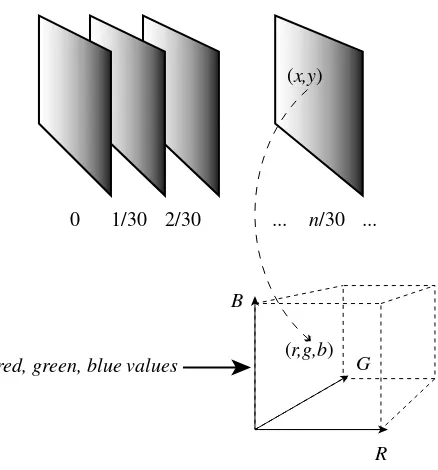
0 1/30 2/30 ... n/30 ...
R B
G
(r,g,b)
red, green, blue values
Figure 1.9: Illustration of the functionAltVideo.
Similarly to figure1.8, we can depictAltVideoas in figure1.9. The RGB value assigned to a point
(x, y)at timetis
(r, g, b) =AltVideo(t, x, y). (1.5)
If the signals specified in (1.4) and (1.5) represent the same video, then for allt∈FrameTimesand
(x, y)∈DiscreteVerticalSpace×HorizontalSpace,
(Video(t))(x, y) =AltVideo(t, x, y). (1.6)
It is worth pausing to understand the notation used in (1.6). Video is a function oft, soVideo(t) is an element in its rangeImageSet. Since elements inImageSet themselves are functions, Video(t) is a function. The domain ofVideo(t) is the product set DiscreteVerticalSpace ×HorizontalSpace, so (Video(t))(x, y) is the value of this function at the point(x, y)in its domain. This value is an element of Intensity3. On the right-hand side of (1.6)AltVideois a function of(t, x, y)and so
1.1.4 Signals representing physical attributes
The change over time in the attributes of a physical object or device can be represented as functions of time or space.
Example 1.3: The position of an airplane can be expressed as
Position:Time→Reals3,
where for allt∈Time,
Position(t) = (x(t), y(t), z(t))
is its position in 3-dimensional space at timet. The position and velocity of the airplane is a function
PositionVelocity:Time→Reals6, (1.7) where
PositionVelocity(t) = (x(t), y(t), z(t), vx(t), vy(t), vz(t)) (1.8) gives its position and velocity att∈Time.
The position of the pendulum shown in the left panel of figure1.10is represented by the function
θ:Time→[−π, π],
whereθ(t)is the angle with the vertical made by the pendulum at timet.
The position of the upper and lower arms of a robot depicted in the right panel of figure
1.10can be represented by the function
(θu, θl):Time→[−π, π]2,
where θu(t) is the angle at the elbow made by the upper arm with the vertical, and θl(t)is the angle made by the lower arm with the upper arm at timet. Note that we can regard(θu, θl)as a single function with range as the product set[−π, π]2or as two functionsθuandθleach with range[−π, π]. Similarly, we can regardPositionVelocity in (1.7) as a single function with rangeReals6 or as a collection of six functions, each with rangeReals, as suggested by (1.8).
Example 1.4: The spatial variation of temperature over some volume of space can be represented by a function
AirTemp:X×Y ×Z →Reals
elbow
θ θu
θl
Figure 1.10: Position of a pendulum (left) and upper and lower arms of a robot (right).
1.1.5 Sequences
Above we studied examples in which temporal or spatial information is represented by functions of a variable representing time or space. The domain of time or space may be continuous as inVoice andImageor discrete as inComputerVoiceandComputerImage.
In many situations, information is represented assequencesof symbols rather than as functions of time or space. These sequences occur in two ways: as a representation ofdataor as a representation of anevent stream.
Examples of data represented by sequences are common. A file stored in a computer in binary form is a sequence of bits, or binary symbols, i.e. a sequence of 0’s and 1’s. A text, like this book, is a sequence of words. A sheet of music is a sequence of notes.
Example 1.5: Consider anN-bit long binary file,
b1, b2,· · ·, bN,
where eachbi ∈Bin={0,1}. We can regard this file as a function File:{1,2,· · ·, N} →Bin,
with the assignmentFile(n) =bnfor everyn∈ {1,· · ·, N}.
If instead ofBinwe take the range to beEnglishWords, then an N-word long English text is a function
EnglishText:{1,2,· · ·, N} →EnglishWords.
In general, data sequences are functions of the form
whereIndices ⊂Nats, whereNatsis the set of natural numbers, is an appropriate index set such as {1,2,· · ·, N}, andSymbolsis an appropriate set of symbols such asBinorEnglishWords.
One advantage of the representation (1.9) is that we can then interpret Data as a discrete-time signal, and so some of the techniques that we will develop in later chapters for those signals will automatically apply to data sequences. However, the domain Indices in (1.9) does not represent uniformly spaced instances of time. All we can say is that ifmandnare inIndiceswithm < n, then them-th symbolData(m)occurs in the data sequencebeforethen-th symbolData(n), but we cannot say how much time elapses between the occurrence of those two symbols.
The second way in which sequences arise is as representations of event streams. Anevent stream ortraceis a record or log of the significant events that occur in a system of interest. Here are some everyday examples.
Example 1.6: When you call someone by phone, the normal sequence of events is
LiftHandset, HearDialTone, DialDigits, HearTelephoneRing, HearCalleeAnswer,· · · but if the other phone is busy, the event trace is
LiftHandset, HearDialTone, DialDigits, HearBusyTone,· · · When you send a file to be printed the normal trace of events is
CommandPrintFile, FilePrinting, PrintingComplete
but if the printer has run out of paper, the trace might be
CommandPrintFile, FilePrinting, MessageOutofPaper, InsertPaper,· · ·
Example 1.7: When you enter your car the starting trace of events might be
StartEngine, SeatbeltSignOn, BuckleSeatbelt, SeatbeltSignOff,· · ·
Thus event streams are functions of the form
EventStream:Indices →EventSet.
We will see in chapter 3 that the behavior of finite state machines is best described in terms of event traces, and that systems that operate on event streams are often best described as finite state machines.
1.1.6 Discrete signals and sampling
it could be a function of a space continuum. We can define a function ComputerVideo where all three sets that are composed to form the domain are discrete.
Discrete signals often arise from signals with continuous domains bysampling. We briefly motivate sampling here, with a detailed discussion to be taken up later. Continuous domains have an infinite number of elements. Even the domain [0,1] ⊂ Time representing a finite time interval has an infinite number of elements. The signal assigns a value in its range to each of these infinitely many elements. Such a signal cannot be stored in a finite digital memory device such as a computer or CD-ROM. If we wish to store, say,Voice, we must approximate it by a signal with a finite domain.
A common way to approximate a function with a continuous domain like Voice and Imageby a function with a finite domain is by uniformly sampling its continuous domain.
Example 1.8: If we sample a 10-second long domain ofVoice,
Voice: [0,10]→Pressure,
10,000 times a second (i.e. at a frequency of 10 kHz) we get the signal
SampledVoice:{0,0.0001,0.0002,· · ·,9.9998,9.9999,10} →Pressure, (1.10) with the assignment
SampledVoice(t) =Voice(t), for allt∈ {0,0.0001,0.0002,· · ·,9.9999,10}. (1.11) Notice from (1.10) that uniform sampling means picking a uniformly spaced subset of points of the continuous domain[0,10].
In the example, thesampling intervalorsampling periodis 0.0001 sec, corresponding to a sam-pling frequencyorsampling rateof 10,000 Hz. Since the continuous domain is 10 seconds long, the domain ofSampledVoicehas 100,000 points. A sampling frequency of 5,000 Hz would give the domain{0,0.0002,· · ·,9.9998,10}, which has half as many points. The sampled domain is finite, and its elements are discrete values of time.
Notice also from (1.11) that the pressure assigned by SampledVoiceto each time in its domain is the same as that assigned byVoiceto the same time. That is,SampledVoiceis indeed obtained by sampling theVoicesignal at discrete values of time.
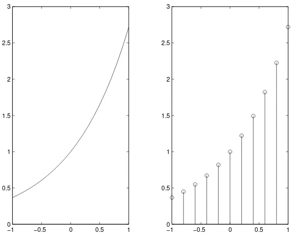
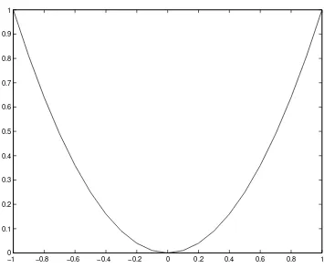
Figure1.11shows an exponential functionExp: [−1,1]→Realsdefined by Exp(x) =ex.
SampledExpis obtained by sampling with a sampling interval of 0.2. So its domain is
−1 −0.5 0 0.5 1 0
0.5 1 1.5 2 2.5 3
−10 −0.5 0 0.5 1
0.5 1 1.5 2 2.5 3
Figure 1.11: The exponential functionsExpandSampledExp, obtained by sampling with a sampling interval of 0.2.
The continuous domain ofImagegiven by (1.1), which describes a grayscale image on an 8.5 by 11 inch sheet of paper, is the rectangle[0,11]×[0,8.5], representing the space of the page. In this case, too, a common way to approximateImageby a signal with finite domain is to sample the rectangle. Uniform sampling with aspatial resolutionof say, 100 dots per inch, in each dimension, gives the finite domainD={0,0.01,· · ·,8.49,8.5} × {0,0.01,· · ·,10.99,11.0}. So the sampled grayscale picture is
SampledImage:D→[0, Bmax] with
SampledImage(x, y) =Image(x, y), for all(x, y)∈D.
As mentioned before, each sample of the image is called apixel, and the size of the image is often given in pixels. The size of your computer screen display, for example, may be 600 ×800 or
768×1024pixels.
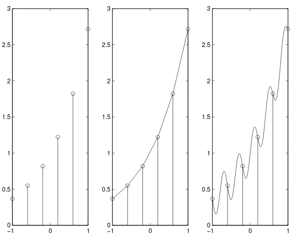
Sampling and approximation
−1 0 1 0
0.5 1 1.5 2 2.5
−1 0 1
0 0.5 1 1.5 2 2.5
−1 0 1
0 0.5 1 1.5 2 2.5
Figure 1.12: The discrete-time signal on the left is obtained by sampling the continuous-time signal in the middle or the one on the right.
For the moment, let us note that the short answer to