Series Editors
Howard Brandt, US Army Research Laboratory, Adelphi, MD, USA Nicolas Gisin, University of Geneva, Geneva, Switzerland
Raymond Laflamme, University of Waterloo, Waterloo, Canada Gaby Lenhart, ETSI, Sophia-Antipolis, France
Daniel Lidar, University of Southern California, Los Angeles, CA, USA Gerard Milburn, University of Queensland, St. Lucia, Australia
Masanori Ohya, Tokyo University of Science, Tokyo, Japan
Arno Rauschenbeutel, Vienna University of Technology, Vienna, Austria Renato Renner, ETH Zurich, Zurich, Switzerland
Maximilian Schlosshauer, University of Portland, Portland, OR, USA Howard Wiseman, Griffith University, Brisbane, Australia
For further volumes:
Quantum Science and Technology
Aims and Scope
Quantum Walks and Search
Algorithms
Department of Computer Science National Laboratory of Scientific
Computing (LNCC) Petr´opolis, RJ, Brazil
ISBN 978-1-4614-6335-1 ISBN 978-1-4614-6336-8 (eBook) DOI 10.1007/978-1-4614-6336-8
Springer New York Heidelberg Dordrecht London
Library of Congress Control Number: 2013930230 © Springer Science+Business Media New York 2013
This work is subject to copyright. All rights are reserved by the Publisher, whether the whole or part of the material is concerned, specifically the rights of translation, reprinting, reuse of illustrations, recitation, broadcasting, reproduction on microfilms or in any other physical way, and transmission or information storage and retrieval, electronic adaptation, computer software, or by similar or dissimilar methodology now known or hereafter developed. Exempted from this legal reservation are brief excerpts in connection with reviews or scholarly analysis or material supplied specifically for the purpose of being entered and executed on a computer system, for exclusive use by the purchaser of the work. Duplication of this publication or parts thereof is permitted only under the provisions of the Copyright Law of the Publisher’s location, in its current version, and permission for use must always be obtained from Springer. Permissions for use may be obtained through RightsLink at the Copyright Clearance Center. Violations are liable to prosecution under the respective Copyright Law.
The use of general descriptive names, registered names, trademarks, service marks, etc. in this publication does not imply, even in the absence of a specific statement, that such names are exempt from the relevant protective laws and regulations and therefore free for general use.
While the advice and information in this book are believed to be true and accurate at the date of publication, neither the authors nor the editors nor the publisher can accept any legal responsibility for any errors or omissions that may be made. The publisher makes no warranty, express or implied, with respect to the material contained herein.
Printed on acid-free paper
This is a textbook aboutquantum walksandquantum search algorithms. The reader will take advantage of the pedagogical aspects of this book and learn the topics faster and make less effort than reading the original research papers, often written in jargon. The exercises and references allow the readers to deepen their knowledge on specific issues. Guidelines to use or to develop computer programs for simulating the evolution of quantum walks are also available.
There is a gentle introduction to quantum walks in Chap.2, which analyzes both the discrete- and continuous-time models on a discrete line state space. Chapter4
is devoted to Grover’s algorithm, describing its geometrical interpretation, often presented in textbooks. It describes the evolution by means of thespectral decom-positionof the evolution operator. The technique calledamplitude amplificationis also presented. Chapters5and6deal with analytical solutions of quantum walks on important graphs: line, cycles, two-dimensional lattices, and hypercubes using the Fourier transform. Chapter7presents an introduction of quantum walks on generic graphs and describes methods to calculate the limiting distribution and the mixing time. Chapter8 describes spatial search algorithms, in special a technique called abstract search algorithm. The two-dimensional lattice is used as example. This chapter also shows how Grover’s algorithm can be described using a quantum walk on the complete graph. Chapter9 introduces Szegedy’s quantum-walk model and the definition of the quantum hitting time. The complete graph is used as example. An introduction to quantum mechanics in Chap.2and an appendix on linear algebra are efforts to make the book self-contained.
in the area of quantum walks, Chap. 4 can be skipped and the focus should be on Chaps.2,5–7. Grover’s algorithm plays an essential role in Chaps.8 and9. Chapter6 is very technical and repetitive. In a first reading, it is possible to skip the analysis of quantum walks on finite lattices and hypercubes in Chap. 6 and in the subsequent chapters. In many passages, the reader must go slow, perform the calculations and fill out the details before proceeding. Some of those topics are currently active research areas with strong impact on the development of new quantum algorithms.
Corrections, suggestions, and comments are welcome, which can be sent through webpage (qubit.lncc.br) or directly to the author by email ([email protected]).
I am grateful to SBMAC, the Brazilian Society of Computational and Applied Mathematics, which publishes a very nice periodical of booklets, called Notes of Applied Mathematics. A first version of this book was published in this collection with the nameQuantum Search Algorithms. I thank SBC, the Brazilian Computer Society, which developed a report called Research Challenges for Computer Science in Brazil that calls attention to the importance of fundamental research on new technologies that can be an alternative to silicon-based computers. I thank the Computer Science Committee of CNPq for its continual support during the last years, providing essential means for the development of this book. I acknowledge the importance of CAPES, which has an active section for evaluating and assessing research projects and graduate programs and has been continually supporting science of high quality, giving an important chance for cross-disciplinary studies, including quantum computation.
I learned a lot of science from my teachers, and I keep learning with my students. I thank them all for their encouragement and patience. There are many more people I need to thank including colleagues of LNCC and the group of quantum computing, friends and collaborators in research projects and conference organization. Many of them helped by reviewing, giving essential suggestions and spending time on this project, and they include: Peter Antonelli, Stefan Boettcher, Demerson N. Gonc¸alves, Pedro Carlos S. Lara, Carlile Lavor, Franklin L. Marquezino, Nolmar Melo, Raqueline A. M. Santos, and Angie Vasconcellos.
1 Introduction . . . 1
2 The Postulates of Quantum Mechanics. . . 3
2.1 State Space. . . 3
2.1.1 State–Space Postulate . . . 5
2.2 Unitary Evolution. . . 6
2.2.1 Evolution Postulate. . . 6
2.3 Composite Systems. . . 9
2.4 Measurement Process. . . 10
2.4.1 Measurement Postulate. . . 10
2.4.2 Measurement in Computational Basis. . . 12
2.4.3 Partial Measurement in Computational Basis. . . 14
3 Introduction to Quantum Walks. . . 17
3.1 Classical Random Walks . . . 17
3.1.1 Random Walk on the Line. . . 17
3.1.2 Classical Discrete Markov Chains. . . 20
3.2 Discrete-Time Quantum Walks. . . 23
3.3 Classical Markov Chains. . . 31
3.4 Continuous-Time Quantum Walks. . . 32
4 Grover’s Algorithm and Its Generalization.. . . 39
4.1 Grover’s Algorithm. . . 39
4.1.1 Analysis of the Algorithm Using Reflection Operators. . . 42
4.1.2 Analysis Using the Spectral Decomposition. . . 46
4.1.3 Comparison Analysis. . . 48
4.2 Optimality of Grover’s Algorithm.. . . 50
4.3 Search with Repeated Elements. . . 55
4.3.1 Analysis Using Reflection Operators. . . 56
4.3.2 Analysis Using the Spectral Decomposition. . . 58
5 Quantum Walks on Infinite Graphs. . . 65
5.1 Line. . . 65
5.1.1 Hadamard Coin. . . 66
5.1.2 Fourier Transform . . . 67
5.1.3 Analytical Solution. . . 71
5.1.4 Other Coins . . . 74
5.2 Two-Dimensional Lattices. . . 75
5.2.1 The Hadamard Coin. . . 78
5.2.2 The Fourier Coin. . . 79
5.2.3 The Grover Coin. . . 79
5.2.4 Standard Deviation . . . 80
5.2.5 Program QWalk. . . 81
6 Quantum Walks on Finite Graphs. . . 85
6.1 Cycle. . . 85
6.1.1 Fourier Transform . . . 87
6.1.2 Analytical Solutions. . . 90
6.1.3 Periodic Solutions . . . 93
6.2 Finite Two-Dimensional Lattice. . . 94
6.2.1 Fourier Transform . . . 96
6.2.2 Analytical Solutions. . . 101
6.3 Hypercube. . . 102
6.3.1 Fourier Transform . . . 105
6.3.2 Analytical Solutions. . . 110
6.3.3 Reducing the Hypercube to a Line. . . 113
7 Limiting Distribution and Mixing Time. . . 121
7.1 Quantum Walks on Graphs. . . 121
7.2 Limiting Probability Distribution . . . 123
7.2.1 Limiting Distribution in the Fourier Basis. . . 128
7.3 Limiting Distribution in Cycles. . . 130
7.4 Limiting Distribution in Hypercubes.. . . 134
7.5 Limiting Distribution in Finite Lattices. . . 137
7.6 Distance Between Distributions. . . 139
7.7 Mixing Time. . . 142
8 Spatial Search Algorithms. . . 145
8.1 Abstract Search Algorithm. . . 145
8.2 Analysis of the Evolution.. . . 151
8.3 Finite Two-Dimensional Lattice. . . 156
8.4 Grover’s Algorithm as an Abstract Search Algorithm. . . 161
8.5 Generalization.. . . 163
9 Hitting Time. . . 165
9.1 Classical Hitting Time. . . 165
9.1.1 Hitting Time Using the Stationary Distribution. . . 167
9.2 Reflection Operators in a Bipartite Graph. . . 171
9.3 Quantum Evolution Operator. . . 174
9.4 Singular Values and Vectors. . . 175
9.5 Spectral Decomposition of the Evolution Operator. . . 177
9.6 Quantum Hitting Time. . . 180
9.7 Probability of Finding a Marked Element. . . 183
9.8 Quantum Hitting Time in the Complete Graph. . . 184
9.8.1 Probability of Finding a Marked Element. . . 189
A Linear Algebra for Quantum Computation . . . 195
A.1 Vector Spaces. . . 195
A.2 Inner Product. . . 196
A.3 The Dirac Notation. . . 197
A.4 Computational Basis. . . 198
A.5 Qubit and the Bloch Sphere. . . 199
A.6 Linear Operators. . . 201
A.7 Matrix Representation. . . 202
A.8 Diagonal Representation.. . . 203
A.9 Completeness Relation. . . 204
A.10 Cauchy–Schwarz Inequality.. . . 204
A.11 Special Operators. . . 205
A.12 Pauli Matrices. . . 207
A.13 Operator Functions.. . . 208
A.14 Tensor Product. . . 210
A.15 Registers. . . 212
References. . . 215
Chapter 1
Introduction
Quantum mechanics has changed the way we understand the physical world and has introduced new ideas that are difficult to accept, not because they are complex, but because they are different from what we are used to in our everyday lives. Those new ideas can be collected in four postulates or laws. It is hard to believe that Nature works according to those laws, and the difficulty starts with the notion of the superposition of contradictory possibilities. Do you accept the idea that a billiard ball could rotate around its axis in both directions at the same time?
Quantum computation was born from this kind of idea. We know that digital classical computers work with zeroes and ones and that the value of the bit cannot be zero and one at the same time. The classical algorithms must obey Boolean logic. So, if the coexistence of bit-0 and bit-1 is possible, which logic should the algorithms obey?
Quantum computation was born from a paradigm change. Information storage, processing and transmission obeying quantum mechanical laws allowed the de-velopment of new algorithms, faster than the classical analogues, which can be implemented in physics laboratories. Nowadays, quantum computation is a well-established area with important theoretical results within the context of the theory of computing, as well as in terms of physics, and has raised huge engineering challenges to the construction of the quantum hardware.
The processing of classical computers is very stable. Depending on the calcula-tion, an inversion of a single bit could invalidate the entire process. But we know that long computations, which require inversion of billions of bits, are performed without problems. Classical computers are error prone because its basic components are stable. Consider, for example, a mechanical computer. It would be very unusual for a mechanical device to change its position, especially if we put a spring to keep it stable in the desired position. The same is true for electronic devices, which remain in their states until an electrical pulse of sufficient power changes this. Electronic devices are built to operate at a power level well above the noise and this noise is kept low by dissipating heat into the environment.
The laws of quantum mechanics require that the physical device must be isolated from the environment, otherwise the superposition vanishes, at least partially. It is a very difficult task to isolate physical systems from their environment. Ultra-relativistic particles and gravitational waves pass through any blockade, penetrate into the most guarded places, obtain information, and convey it out of the system. This process is equivalent to a measurement of a quantum observable, which often collapses the superposition and slows down the quantum computer, making it almost, or entirely, equivalent to the classical one. Techniques for signal amplification and noise dissipation cannot be applied to quantum devices in the same way they are used in conventional devices. This fact raises questions about the feasibility of quantum computers. On the other hand, theoretical results show that there are no fundamental issues against the possibility of building quantum hardware. Researchers say that it is only a matter of technological difficulty.
Chapter 2
The Postulates of Quantum Mechanics
It is impossible to present quantum mechanics in a few pages. Since the goal of this book is to describe quantum algorithms, we limit ourselves to theprinciplesof quantum mechanics and describe them as “game rules.” Suppose you have played checkers for many years and know several strategies, but you really do not know chess. Suppose now that someone describes the chess rules. Soon you will be playing a new game. Certainly, you will not master many chess strategies, but you will be able to play. This chapter has a similar goal. The postulates of a theory are its game rules. If you break the rules, you will be out of the game.
At best, we can focus on four postulates. The first describes the arena where the game goes on. The second describes the dynamics of the process. The third describes how we adjoin various systems. The fourth describes the process of physical measurement. All these postulates are described in terms of linear algebra. It is essential to have a solid understanding of the basic results in this area. Moreover, the postulate of composite systems uses the concept of tensor product, which is a method of combining two vector spaces to build a larger vector space. It is also important to be familiar with this concept.
2.1
State Space
Z
A
B O
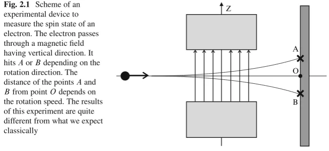
Fig. 2.1 Scheme of an experimental device to measure the spin state of an electron. The electron passes through a magnetic field having vertical direction. It hitsAorBdepending on the rotation direction. The distance of the pointsAand
Bfrom pointOdepends on the rotation speed. The results of this experiment are quite different from what we expect classically
ball is spinning and whose length characterizes the speed of rotation. In classical physics, the direction of the rotation axis can vary continuously, as well as the rotation intensity.
Does anelectron, which is considered an elementary particle,i.e.not composed of other smaller particles, rotates like a billiard ball? The best way to answer this is by experimenting in real settings to check whether the electron in fact rotates and whether it obeys the laws of classical physics. Since the electron has charge, its rotation would produce magnetic fields that could be measured. Experiments of this kind were performed at the beginning of quantum mechanics, with beams of silver atoms, later on with beams of hydrogen atoms, and today they are performed with individual particles (instead of beams), such as electrons or photons. The results are different from what is expected by the laws of the classical physics.
We can send the electron through a magnetic field in the vertical direction (directionz), according to the scheme of Fig.2.1. The possible results are shown. Either the electron hits the screen at the pointAor pointB. One never finds the electron at pointO, which means no rotation. This experiment shows that thespin of the electron only admits two values:spin upandspin downboth with the same intensity of “rotation.” This result is quite different from classical, since the direction of the rotation axis is quantized, admitting only two values. The rotation intensity is also quantized.
Quantum mechanics describes the electron spin as a unit vector in the Hilbert spaceC2. Thespin upis described by the vector
j0i D
1 0
andspin downby the vector
j1i D
0 1
This seems a paradox, because vectors j0i and j1i are orthogonal. Why use orthogonal vectors to describespin upandspin down? InR3, if we addspin upand spin down, we obtain a rotationless particle, because the sum of two opposite vectors of equal length gives the zero vector, which describes the absence of rotation. In the classical world, you cannot rotate a billiard ball to both sides at the same time. We have two mutually excluded situations. It is thelaw of excluded middle. The notions of spin upandspin down refer toR3, whereas quantum mechanics
describes the behavior of the electron before the observation, that is, before entering the magnetic field, which aims to determine its state of rotation.
If the electron has not entered the magnetic field and if it is somehow isolated from the macroscopic environment, its spin state is described by a linear combina-tion of vectorsj0iandj1i
j i Da0j0i Ca1j1i; (2.1) where the coefficientsa0anda1are complex numbers that satisfy the constraint
ja0j2C ja1j2D1: (2.2) Since vectorsj0iandj1iare orthogonal, the sum does not result in the zero vector. Excluded situations in classical physics can coexist in quantum mechanics. This coexistence is destroyed when we try to observe it using the device shown in Fig. 2.1. In the classical case, the spin state of an object is independent of the choice of the measuring apparatus and, in principle, has not changed after the measurement. In the quantum case, the spin state of the particle is a mathematical idealization which depends on the choice of the measuring apparatus to have a physical interpretation and, in principle, suffers irreversible changes after the measurement. The quantities ja0j2 andja1j2 are interpreted as the probability of detection of spin up or down, respectively.
2.1.1
State–Space Postulate
Anisolated physical systemhas an associated Hilbert space, called thestate space. The state of the system is fully described by a unit vector, called thestate vectorin that Hilbert space.
Notes
2. A system is isolated orclosedif it does not influence and is not influenced by the outside. In principle, the system need not be small, but it is easier to isolate small systems with few atoms. In practice, we can only deal with approximate isolated systems, so the state–space postulate is an idealization.
The state–space postulate is impressive, on the one hand, but deceiving, on the other hand. The postulate admits that classically incompatible states coexist in superposition, such as rotating to both sides simultaneously, but this occurs only in isolated systems,i.e.we cannot see this phenomenon, as we are on the outside of the insulation (let us assume that we are notSchr¨odinger’s cat). A second restriction demanded by the postulate is that quantum states must have unit norm. The postulate constraints show that the quantum superposition is not absolute, i.e. is not the way we understand the classical superposition. If quantum systems admit a kind of superposition that could be followed classically, the quantum computer would have available an exponential amount of parallel processors with enough computing power to solve the problems inclass NP-complete.1It is believed that the quantum computer is exponentially faster than the classical computer only in a restricted class of problems.
2.2
Unitary Evolution
The goal of physics is not simply to describe the state of a physical system at a given time, rather the main objective is to determine the state of this system in future. A theory makes predictions that can be verified or falsified by physical experiments. This is equivalent to determining the dynamical laws the system obeys. Usually, these laws are described by differential equations, which govern the time evolution of the system.
2.2.1
Evolution Postulate
Thetime evolutionof an isolated quantum system is described by aunitary trans-formation. If the state of the quantum system at timet1is described by vectorj 1i, the system statej 2iat timet2is obtained fromj 1iby a unitary transformationU, which depends only ont1andt2, as follows:
j 2i D Uj 1i: (2.3)
A B
2 1
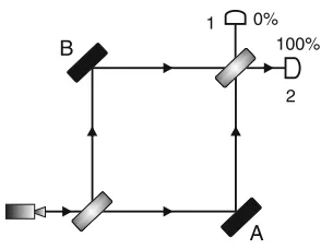
100% 0% Fig. 2.2 Schematic drawing
of an experimental device, which consists of a light source, two half-silvered mirrors A and B, fully reflective mirrors, detectors 1 and 2. The interference produced by the last half-silvered mirror makes all light to go to the detector 2
Notes
1. The action of a unitary operator on a vector preserves its norm. Thus, ifj iis a unit vector,Uj iis also a unit vector.
2. Aquantum algorithmis a prescription of a sequence of unitary operators applied to an initial state takes the form
j ni DUn U1j 1i:
The qubits in state j ni are measured, returning the result of the algorithm. Before measurement, we can obtain the initial state from the final state because unitary operators are invertible.
3. The evolution postulate is to be written in the form of a differential equation, calledSchr¨odinger equation. This equation provides a method to obtain operator U once given the physical context. Since the goal of physics is to describe the dynamics of physical systems, the Schr¨odinger equation plays a fundamental role. The goal of computer science is to analyze and implement algorithms, so the computer scientist wants to know if it is possible to implement some form of a unitary operator previously chosen. Equation (2.3) is useful for the area of quantum algorithms.
interference with the beam going to the detector 1 and constructive interference with the beam going to the detector 2. However, if the light intensity emitted by the source is decreased such that one photon is emitted at a time, this explanation fails. If we insist on using classical physics in this situation, we predict that 50% of the photons would be detected by detector 1 and 50% by detector 2, because the photon either goes through the mirror A or goes through B, and it is not possible to interfere since it is a single photon.
Inquantum mechanics, if the set of mirrors is isolated from the environment, the two possible paths are represented by two orthonormal vectors j0i and j1i, which generate the state space that describes the possible paths to reach the photon detector. Therefore, a photon can be in superposition of “path A,” described byj0i, together with “path B,” described byj1i. This is the application of the first postulate. The next step is to describe the dynamics of the process. How is this done and what are the unitary operators in the process? In this experiment, the dynamics is produced by the half-silvered mirrors, since they generate the paths. The action of the half-silvered mirrors on the photon must be described by a unitary operatorU. This operator must be chosen so that the two possible paths are created in a balanced way,i.e.
Uj0i D j0i Ce ij1i p
2 : (2.4)
This is the most general case where paths A and B have the same probability to be followed, because the coefficients have the same modulus. To complete the definition of operatorU, we need to know its action on statej1i. There are many possibilities, but the most natural choice that reflects the experimental device is
D=2and
U D p1 2
1 i i 1
: (2.5)
The state of the photon after passing through the second half-silvered mirror is
U.Uj0i/D .j0i Cij1i/Ci.ij0i C j1i/ 2
Dij1i: (2.6)
2.3
Composite Systems
Thepostulate of composite systemsstates that the state space of acomposite system is thetensor productof the state space of the components. Ifj 1i; : : :,j nidescribe the states of n isolated quantum systems, the state of the composite system is j 1i ˝ ˝ j ni.
An example of a composite system is the memory of a n-qubit quantum computer. Usually, the memory is divided into sets of qubits, called registers. The state space of the computer memory is the tensor product of the state space of the registers, which is obtained by repeated tensor product of the Hilbert space
C2of eachqubit.
The state space of the memory of a 2-qubit quantum computer isC4DC2˝C2. Therefore, any unit vector inC4 represents the quantum state of two qubits. For example, the vector
j0; 0i D 2 6 6 4 1 0 0 0 3 7 7
5; (2.7)
which can be written asj0i ˝ j0i, represents the state of two electrons both with spin up. Analogous interpretation applies toj0; 1i,j1; 0i, andj1; 1i. Consider now the unit vector inC4given by
j i D j0; 0i C jp 1; 1i
2 : (2.8)
What is the spin state of each electron in this case? To answer this question, we have to factorj ias follows:
j0; 0i C j1; 1i p
2 D
aj0i Cbj1i˝cj0i Cdj1i: (2.9)
We can expand the right-hand side and match the coefficients setting up a system of equations to finda,b,c, andd. The state of the first qubit will beaj0i Cbj1iand second will becj0i Cdj1i. But there is a big problem: the system of equations has no solution,i.e.there are no coefficientsa,b,c, anddsatisfying (2.9). Every state of a composite system that cannot be factored is calledentangled. The quantum state is well defined when we look at the composite system as a whole, but we cannot attribute the states to the parts.
Exercise 2.1. Consider the states j 1i D
1 2
j0; 0i j0; 1i C j1; 0i j1; 1i;
j 2i D 1 2
j0; 0i C j0; 1i C j1; 0i j1; 1i: Show thatj 1iis not entangled andj 2iis entangled.
Exercise 2.2. Show that if j i is an entangled state of two qubits, then the application of a unitary operator of the formU1 ˝U2 necessarily generates an entangled state.
2.4
Measurement Process
In general, measuring a quantum system that is in the state j iseeks to obtain classical information about this state. In practice, measurements are performed in laboratories using devices such as lasers, magnets, scales, and chronometers. In theory, we describe the process mathematically in a way that is consistent with what occurs in practice. Measuring a physical system that is in an unknown state, in general, disturbs this state irreversibly. In those cases, there is no way to know or recover the state before the measurement. If the state was not disturbed, no new information about it is obtained. Mathematically, the disturbance is described by a orthogonal projector. If the projector is over an one-dimensional space, it is said that the quantum statecollapsedand is now described by the unit vector belonging to the one-dimensional space. In the general case, the projection is over a vector space of dimension greater than 1, and it is said that the collapse is partial or, in extreme cases, there is no change at all in the quantum state of the system.
The measurement requires the interaction between the quantum system with a macroscopic device, which violates thestate–space postulate, because the quantum system is not isolated at this moment. We do not expect the evolution of the quantum state during the measurement process to be described by a unitary operator.
2.4.1
Measurement Postulate
Aprojective measurementis described by a Hermitian operatorO, called observ-able in the state space of the system being measured. The observableO has a diagonal representation
O D X
P; (2.10)
If the system state at the time of measurement isj i, the probability of obtaining the resultwill bekPj ik2or, equivalently,
p D h jPj i: (2.11)
If the result of the measurement is, the state of the quantum system immediately after the measurement will be
1 pp
Pj i: (2.12)
Notes
1. There is a correspondence between the physical layout of the devices in a physics lab and the observableO. When an experimental physicist measures a quantum system, she or he gets real numbers as result. Those numbers correspond to the eigenvaluesof the Hermitean operatorO.
2. The statesj iand eij ihave the sameprobability distributionpwhen one measures the same observable O. The states after measurement differ by the same factor ei. The term ei multiplying a quantum state is calledglobal phase factorwhereas a term eimultiplying a vector of a sum of vectors, such as j0i Ceij1i, is calledrelative phase factor. The real numberis calledphase. Since the possible outcomes of a measurement of observableOobey a probabil-ity distribution, we can define theexpected valueof a measurement as
hOi D X
p; (2.13)
and thestandard deviationas
ODphO2i hOi2: (2.14) It is important to remember that the mean and standard deviation of an observable depends on the state that the physical system was in just before the measurement. Exercise 2.3. Show thathOi D h jOj i:
Exercise 2.4. Show that if the physical system is in a statej ithat is an eigenvector of O, then O D 0, that is, there is no uncertainty about the result of the measurement of the observableO. What is the result of the measurement?
Exercise 2.5. Show thatPp D1for any observableOand any statej i. Exercise 2.6. Suppose that the physical system is in generic statej i. Show that P
2.4.2
Measurement in Computational Basis
The computational basis of space C2 is the set ˚j0i; j1i. For one qubit, the observable of themeasurement in the computational basisis Pauli matrixZ, whose spectral decomposition is
Z D .C1/PC1C.1/P1; (2.15) wherePC1 D j0ih0jandP1 D j1ih1j. The possible results of the measurement are˙1. If the state of the qubit is given by (2.1), the probabilities associated with possible outcomes are
pC1D ja0j2; (2.16) p1D ja1j2; (2.17) whereas the states immediately after the measurement arej0iandj1i, respectively. In fact, each of these states has a global phase that can be discarded. Note that
pC1Cp1D1; because statej ihave unit norm.
Before generalizing ton qubits, it is interesting to reexamine the process of measurement of a qubit with another observable given by
OD
1 X
kD0
kjkihkj: (2.18)
Since the eigenvalues ofO are 0 and 1, the above analysis holds if we replaceC1 by 0 and1by 1. With this new observable, there is a one-to-one correspondence in the nomenclature of the measurement result and the final state. If the result is 0, the state after the measurement isj0i. If the result is 1, the state after the measurement isj1i.
The computational basisof the Hilbert space of n qubits in decimal notation is the set ˚j0i; : : : ; j2n1i. The measurement in the computational basis is associated with observable
OD
2n1 X
kD0
k Pk; (2.19)
wherePkD jkihkj. A generic state ofnqubits is given by
j i D 2n1 X
kD0
where amplitudesaksatisfying the constraint X
k
jakj2D1: (2.21)
The measurement result is an integer valuekin the range0 k 2n1with a probability distribution given by
pkD ˝ ˇˇ
Pk ˇ ˇ ˛
Dˇˇ ˝kˇˇ ˛ ˇˇ2
D jakj2: (2.22)
Equation (2.21) ensures that the sum of the probabilities is 1. The n-qubit state immediately after the measurement is
Pkj i pp
k ' j
ki: (2.23)
For example, suppose that the state of two qubits is given by
j i D p1
3.j0; 0i ij0; 1i C j1; 1i/ : (2.24) The probability that the result is 00, 01 or 11 in binary notation is 1=3. Result 10 is never obtained, because the associated probability is 0. If the measurement result is 00, the system state immediately after will bej0; 0i. Similarly for 01 and 11. For the measurement in the computational basis, it makes sense that the result isstatej0; 0i, because there is a correspondence between eigenvalue 00 and state j0; 0i.
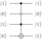
The description of the measurement process of observable (2.19) is equivalent to simultaneous measurements or in a cascade of observablesZ,i.e.one observable Z for each qubit. The possible results of measuring Z are ˙1. Simultaneous measurements, or in a cascade of n qubits, result in a sequence of values ˙1. The relationship between a result of this kind and the one described before is obtained by replacingC1 by0and1 by1. We will have a binary number that can be converted into a decimal number which is one of the valueskof (2.19).
For example, for3qubits the result may be.1;C1;C1/, which is equivalent to .1; 0; 0/. Converting to base ten, we get number 4. The state after the measurement will be obtained using the projector
P1;C1;C1 D j1ih1j ˝ j0ih0j ˝ j0ih0j
D j1; 0; 0ih1; 0; 0j (2.25)
over the state system of the three qubits followed byrenormalization. The renormal-ization in this case replaces the coefficient by 1. The state after measurement will be j1; 0; 0i. So far using the computational basis, for both observables (2.19) andZ’s, we can simply say that the result isj1; 0; 0i, because we automatically know that the eigenvalues ofZin question are.1;C1;C1/and the numberkis 4.
A simultaneous measurement ofn observablesZ is not equivalent to measure observableZ˝ ˝Z. The latter observable returns a single value, which can beC1 or1, whereas withnobservablesZ, simultaneously or not, we obtainnvalues˙1. Measurements on a cascade are performed with observableZ˝I ˝ ˝I,I ˝ Z˝ ˝I, and so on. They can also be performed simultaneously. Usually, we use a more compact notation,Z1,Z2, successively, whereZ1 means that observable Z was used for the first qubit and the identity operator for the remaining qubits. Since these observables commute, the order is irrelevant and the limits imposed by theuncertainty principledo not apply. Measurement of observables of this kind is calledpartial measurementin the computational basis.
Exercise 2.7. Suppose that the state of a qubit isj1i.
1. What is the mean value and standard deviation of the measurement of observ-ableX?
2. What is the mean value and standard deviation of the measurement of observable Z? Compare with Exercise2.4.
2.4.3
Partial Measurement in Computational Basis
j i D r
2 3j0i ˝
j0i ij1i p
2 C
1 p
3j1i ˝ j1i: (2.26) We can see that the measurement result is either 0 or 1. The probability of obtaining 1 is1=3, because the only way to get 1 for a measurement of the first qubit is to obtain 1 as well, for the second qubit. Therefore, the probability of obtaining 0 is 2=3, and the state immediately after the measurement in this case is
j0i ˝ j0i pij1i
2 :
Only the qubits involved in the measurement are projected on the computational basis. The states that have 0 in the first qubit survive and the final state must be renormalized. The remaining qubits may be in superposition. In this example, when the result is 0, the state of the second qubit is a superposition, when the result is 1, the state of the second qubit isj1i.
If we have a system composed of subsystemsAandB, a partial measurement is a measurement of an observable of the typeOA˝IB, whereOAis an observable of systemAandIBis the identity operator of systemB. Physically, this means that the measuring apparatus interacted only with the subsystemA. Equivalently, a partial measurement interacting only with subsystemBis a measurement of an observable of the typeIA˝OB.
If we have a register ofmqubits together with a register ofn qubits, we can represent the computational basis in a compact form ˚ji; ji W0 i 2m 1, 0 j 2n1, wherei andj are both represented in base ten. A generic state will be represented by
j i D 2m1
X
iD0 2n1
X
jD0
aijji; ji: (2.27)
Suppose we measure all qubits of the first register in the computational basis,i.e. we measure observableOA˝IB, where
OAD 2m1
X
kD0
kPk: (2.28)
The probability of obtaining value0k2m1is pkD h j.Pk˝I /j i
D 2n1 X
jD0 ˇ ˇakj
ˇ ˇ2
The set˚p0; : : : ; p2m1is a probability distribution and therefore satisfies 2Xm1
kD0
pk D 1: (2.30)
If the measurement result isk, the state immediately after the measurement will be
1 pp
k
.Pk˝I /j i D 1 pp
kj ki
0 @
2n1 X
jD0 akjjji
1
A: (2.31)
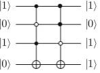
Note that the state after the measurement is a superposition of the second reg-ister. A measurement of observable (2.28) is equivalent to measure observables Z1,: : :,Zm.
Exercise 2.8. Suppose that the state of two qubits is given by
j i D 3
5p2j0; 0i 3 i
5p2j0; 1i C 2p2
5 j1; 0i 2p2 i
5 j1; 1i: (2.32)
1. Describe completely the measurement process of observableZ1, that is, obtain the probability of each outcome and the corresponding states after the measure-ment. Suppose that, after measuringZ1, we measureZ2. Describe all resulting cases.
2. Now invert the order of the observable and describe the whole process.
3. If the intermediate quantum states are disregarded, is there a difference when we invert the order of the observable? Note that the measurement ofZ1andZ2 may be performed simultaneously. One can move the qubits without changing the quantum state, which may be entangled or not, and put each of them into a measuring device, both adjusted to measure observableZ, as in Fig.2.1. 4. For two qubits, the state after the measurement of the first qubit in the
computational basis can be eitherj0ij˛iorj1ijˇi, wherej˛iandjˇiare states of the second qubit. In general, we havej˛i ¤ jˇi. Why is this not the case in previous items?
Further Reading
Chapter 3
Introduction to Quantum Walks
Quantum walksplay an important role in the development of quantum algorithms. Algorithms based on quantum walks generally use a technique called amplitude amplification, which was introduced in Grover’s algorithm. This technique differs from the ones used in algebraic algorithms, in which the Fourier transform plays the main role. However, it is possible to go beyond Grover’s algorithm in terms of efficiency. The best algorithm to solve theelement distinctness problemis based on quantum walks. This problem consists in determining whether there are repeated elements in a set of elements. When Grover’s algorithm is used, the solution is less efficient.
Before describing the area of quantum walks, we will briefly review the area ofclassical random walks with a focus on theexpected distance from the origin induced by theprobability distribution. We will compare the results to thequantum expected distance. We will see that the probability of finding the walker away from the origin is greater in the quantum case. This fact is the main reason why algorithms based on quantum walks can be faster than those based on classical random walks.
3.1
Classical Random Walks
3.1.1
Random Walk on the Line
t n
-5 -4 -3 -2 -1 0 1 2 3 4 5
0 1
1 1
2
1 2
2 1
4
1 2
1 4
3 1
8
3 8
3 8
1 8
4 1
16
1 4
3 8
1 4
1 16
5 1
32
5 32
5 16
5 16
5 32
1 32
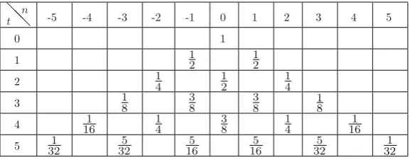
Fig. 3.1 Probability of the particle being in the positionnat timet, assuming it starts the random walk at the origin. The probability is zero in empty cells
Fig. 3.2 Probability distribution of the random walk in a classical one-dimensional lattice for
tD72,tD180andtD450
with probability1=2or inn D 1with probability1=2. The probability of it being in the positionn D 0 becomes zero. Following this reasoning, we can confirm all probabilities described in the table in Fig.3.1.
A generic term in this table is given by
p.t; n/D 1 2t
t tCn
2 !
; (3.1)
distribution of points, because the probability is zero for odd values ofnwhent is even. Another way to interpret the curves of the figure is as the sump.t; n/Cp.tC 1; n/,i.e.we have two overlapping distributions.
We can see in Fig.3.2that the height of the midpoint of the curve decreases as a function of time, whereas the width increases. It is natural to ask what theexpected distancefrom the origin induced by the probability distribution is. It is important to determine how far away from the origin we can find the particle as time goes on. The expected distance is a statistical quantity that captures this idea and is equal to theposition standard deviationwhen the probability distribution is symmetrical. Theaverage position(orexpected position) is
hni D 1
X
nD1
n p.t; n/
D0; (3.2)
it follows that the standard deviation of the probability distribution is q
hn2i hni2 D
v u u t X1
nD1
n2p.t; n/
Dpt : (3.3)
Another way to calculate the standard deviation is by converting the binomial distribution into an expression that is easier to handle analytically. By expanding the binomial factor of (3.1) in terms of factorials, and using Stirling’s approximation for large values of t, the probability distribution of the random walk can be approximated by the expression
p .t; n/' p2 2 te
n2
2t: (3.4)
For a fixed value oftand without the factor 2 in the numerator, this function is called Gaussianornormal distribution. The width of the normal distribution is defined as half the distance between the inflection points. By equating the second derivative @2p=@n2to zero, we eventually obtain the widthpt. The standard deviation is the width of the normal distribution.
Exercise 3.2. The goal of this exercise is to help the calculation of the sum in (3.3). Change the dummy index to obtain a finite sum starting atnD 0and running over even values ofnwhent is even and running over odd values ofn whent is odd. After that you can use (3.1). Rename the dummy index in order to use the identities
t X
nD0 2t
n !
D22t1C1 2
2t t
! ;
t X
nD0 n 2t
n !
Dt 22t1;
t X
nD0 n2 2t
n !
Dt222t1Ct 22t2t 2
2 2t
t !
and simplify the result to show that
1
X
nD1
n2p.t; n/Dt:
Exercise 3.3. Show that (3.4) can be obtained from (3.1) throughStirling’s approx-imation, which is given by
t Šp2 t ttet;
whent 1:Hint: Use Stirling’s approximation and simplify the result trying to factor out the fractionn=t. Take thenatural logarithmof the expression, expand the logarithm, and use the asymptotic expansion of the logarithm. Note that terms of the typen2=t2are much smaller thann2=t. At the end, take the exponential of the result.
3.1.2
Classical Discrete Markov Chains
Aclassical Markov chainis a stochastic process that assumes values in a discrete set and obeys the following property: the next state of the chain only depends on the current state, i.e. it is not influenced by the past states. The Markov chain can be viewed as a directed graph where the states are represented by vertices and directed edges indicate what the possible next states are. The next state is randomly determined. Note that the set of states is discrete, whereas the evolution can be discrete or continuous. Therefore, the term discrete or continuous in this area only refers to time.
(jXj Dn) and set of edgesE. The probability distribution is described by a vector of the form
2 6 4
p1.t / :: : pn.t /
3 7 5;
wherep1.t /is the probability of the walker being at vertexx1at timet. Similarly for the other entries. If the process begins with the walker in the first vertex, we havep1.0/ D 1andpi.0/ D 0fori D 2; : : : ; n. In a Markov chain, we cannot precisely tell where the walker will be in the future. However, we can determine the probability distribution, if we know thetransition matrixM, also calledprobability matrixorstochastic matrix.
If the probability distribution is known at the timet, we obtain the distribution at timetC1by employing the formula
pi.tC1/D n X
jD1
Mi jpj.t /: (3.5)
To ensure thatpi.tC1/is a probability distribution,i.e.pi 0,8iand P
ipi D1, matrixMmust satisfy the following properties: the entries must be nonnegative real numbers and the sum of the entries of any column must be equal to 1. In vector form, we have
E
p.tC1/DM p.t /: (3.6)
Because the matrix is in the left position, this version is calledleft stochastic matrix. There is a corresponding description that uses a transposed vector of probabilities (row vector) and the matrix is on the right position. In this case, the sum of the entries of each line ofM should result in one.
The entryMij of the stochastic matrix is the probability of the walker, who is in vertexxj, to go to vertexxi. The simplest case is when the graph is undirected and
Mij D 1 dj ;
wheredj is the degree orvalence of vertexxj. If there is no edge from xj to xi, then Mij D 0. In this case, the walker goes to one of the adjacent vertices and transition probability is the same for all of them. The stochastic matrix is related to theadjacency matrix.A/of the graph by formulaMij DAij=dj. The adjacency matrix of an undirected graph is a symmetric Boolean matrix specifying whether two verticesxi andxj are connected (entryAij is 1) or not (entryAij is 0).
The vertices do not haveloops, soMi i D0,8i. The stochastic matrix is
M D 1
n1 2 6 6 6 6 6 4
0 1 1 1 1 0 1 1 1 1 0 1
::
: ::: ::: : :: ::: 1 1 1 0 3 7 7 7 7 7 5 : (3.7)
If the initial condition is a walker located on the first vertex, the probability distributions in the first steps will be
E p.0/D 2 6 6 6 4 1 0 :: : 0 3 7 7 7
5; p.1/E D 1 n1
2 6 6 6 4 0 1 :: : 1 3 7 7 7
5; p.2/E D 1 .n1/2
2 6 6 6 4
n1 n2
:: : n2
3 7 7 7 5:
The probability distribution at a generic steptis
E p.t /D
2 6 6 6 4
fn.t1/ fn.t /
:: : fn.t /
3 7 7 7
5; (3.8)
where functionfn.t /is
fn.t /D 1 n
1 1
.1n/t
: (3.9)
Note that whent ! 1, the probability distribution goes to the uniform distribution, which is thelimiting distributionof this graph.
As motivation for the next section, we make some observations about the dynamical structure of discrete Markov chains. Equation (3.6) is a recursive equationthat can be solved and written as
E
p.t /DMtp.0/;E (3.10)
evolutions and describe them in a matrix structure, despite the fact that we know only one possibility actually occurs in a specific situation. The matrix structure of the stochastic evolution will be used in the next section to describe the quantum evolution. However, the physical interpretation of what happens at the physical level is clearly different from the actual stochastic process, since in the quantum case it is not correct to say that only one of the possibilities occurs. From the mathematical point of view, there is a radical change, because the evolution matrix is not applied directly to the probability distribution and the matrix entries need not be positive real numbers. In the quantum case, the matrix entries can be negative or complex numbers and the evolution matrix is applied to the vector ofprobability amplitudes. Exercise 3.4. The purpose of this exercise is to obtain the expression (3.8). By inspecting the stochastic matrix of the complete graph, show thatp2.t /Dp3.t /D Dpn.t /andp1.tC1/Dp2.t /. Considering that the sum of entries of the vector of probabilities is1, show thatp2.t /satisfies the following recursive equation:
p2.t /D
1p2.t1/
n1 :
Using thatp2.0/D0, solve the recursive equation and show thatp2.t /is given by fn.t /, as in (3.9).
Exercise 3.5. Obtain an expression forMt in terms of functionf
n.t /, whereM is the stochastic matrix of the complete graph. From theMt expression, show that
E
p.t /obeys (3.8).
Exercise 3.6. Consider a cycle withnvertices and take as initial condition a walker located in one of the vertices. Obtain the stochastic matrix of this graph. Describe the probability distribution for the first steps and compare to the values in Fig.3.1. Obtain the distribution at a generic time and find the limiting distribution for the odd cycle.Hint: To find the distribution for the cycle, use the probability distribution of the line.
Exercise 3.7. LetM be a generic stochastic matrix. Show thatMt is a stochastic matrix for any positive integert.
3.2
Discrete-Time Quantum Walks
spaces of the components. As the evolution of isolated quantum systems is unitary, there is no room forrandomness. Therefore, in principle, the namequantum random walkis contradictory. In literature, the termquantum walkhas been used instead, but quantum systems that are not totally isolated from the environment may have randomness. In addition, at some point we measure the quantum system to obtain information about it. This process generates a probability distribution.
The first model of quantization of classical random walks that we will discuss is thediscrete-time modelor simplydiscrete model. In the quantum case, the walker’s position n should be a vector in a Hilbert space HP of infinite dimension, the computational basis of which is˚jni W n 2 Z. The evolution of the walk should
depend on a quantum “coin.” If one obtains “heads” after tossing the “coin” and the walker is described by vectorjni, then in the next step it will be described by jnC1i. If it is “tails,” it will be described byjn1i. How do we include the “coin” in this scheme? We can think in physical terms. Suppose an electron is the “random” walker on a one-dimensional lattice. The state of the electron is described not only by its position in the lattice but also by the value of its spin, which may be spin up or spin down. Thus, the spin value can determine the direction of motion. If the electron is in positionjniand its spin is up, it should go tojnC1ikeeping the same spin value. Similarly, when its spin is down, it should gojn1i. The Hilbert space of the system should beHDHC ˝HP, whereHC is the two-dimensional Hilbert space associated with the “coin,” the computational basis of which is˚j0i;j1i. We can now define the “coin” as any unitary matrix C with dimension2, which acts on vectors in Hilbert spaceHC. It is calledcoin operator.
The shift fromjnitojnC1iorjn1imust be described by a unitary operator, called theshift operatorS. It should operate as follows:
Sj0ijni D j0ijnC1i; (3.11) Sj1ijni D j1ijn1i: (3.12) If we know the action ofS on the computational basis ofH, we have a complete description of this linear operator. Therefore, we can deduce that
S D j0ih0j ˝ 1
X
nD1
jnC1ihnj C j1ih1j ˝ 1
X
nD1
jn1ihnj: (3.13)
j .0/i D j0ijnD0i; (3.14) wherej .0/idenotes the state at the initial time andj .t /idenotes the state of the quantum walk at timet.
The coin used for most one-dimensional quantum walks is the Hadamard operator
H D p1 2
1 1 11
: (3.15)
One step consists of applyingH in the state of the coin,i.e.applyingH˝I, where Iis the identity operator of the Hilbert spaceHP, followed by the application of the shift operatorS:
j0i ˝ j0iH!˝I j0i C jp 1i 2 ˝ j0i S
! p1 2
j0i ˝ j1i C j1i ˝ j1i: (3.16)
The result is a superposition of the particle both in positionnD 1and in position n D 1. The superposition of positions is a result of the superposition generated by the coin operator. We can see that the coinH is non-biased when applied toj0i, since the amplitude of the right part is equal to the amplitude of the left part. If we applyH toj1i, there is a sign difference between the amplitudes of the right and left parts. When we calculate the probability of finding the particle at positionn, the sign plays no role. So we can callHa non-biased coin.
What is the next step? In the quantum case, we need to measure the quantum system in the state (3.16) to know what the position of the particle is. If we measure it using the computational basis of HP, we will have a 50% chance of finding the particle at position n D 1 and a 50% chance of finding it at the position n D 1. This result is the same, compared to the first step of the classical random walk. If we repeat the same procedure successively,i.e. (1) we apply the coin operator, (2) we apply the shift operator, and (3) we measure using the computational basis, we will re-obtain the classical random walk. Our goal is to use quantum features to obtain new results, which cannot be obtained in the classical context. When we measure the particle position after the first step, we destroy the correlations between different positions, which are typical of quantum systems. If we do not measure and apply the coin operator followed by the shift operator successively, the quantum correlations between different positions can have constructive or destructive interference, effectively generating a behavior different from the classical context, which is a characteristic of quantum walks. We will see that the probability distribution does not go to the normal distribution and the standard deviation is notpt.
The quantum walk consists in applying the unitary operator
t n
−5 −4 −3 −2 −1 0 1 2 3 4 5
0 1
1 1
2
1 2
2 1
4
1 2
1 4
3 1
8
1 8
5 8
1 8
4 1
16
1 8
1 8
5 8
1 16
5 1
32
5 32
1 8
1 8
17 32
1 32
Fig. 3.3 Probability of finding the quantum particle in positionnat timet, assuming that the walk starts at the origin with the quantum coin in “heads” state
a number of times without intermediate measurements. One step consists in applyingU one time, which is equivalent to applying the coin operator followed by the shift operator. In the next step, we apply U again without intermediate measurements. A timet, the state of the quantum walk is given by
j .t /i DUtj .0/i: (3.18)
Let us calculate the initial steps explicitly to compare with the classical random walk. We will take (3.14) as initial condition. The first step will be equal to (3.16). The second step can be calculated using the formulaj .2/i DUj .1/iand so on.
j .1/i D p1 2
j1ij1i C j0ij1i
j .2/i D 1 2
j1ij2i C.j0i C j1i/j0i C j0ij2i
j .3/i D 1 2p2
j1ij3i j0ij1i C.2j0i C j1i/j1i C j0ij3i
(3.19)
These few initial steps have already revealed that the quantum walk differs from the classical random walk in several aspects. We use a non-biased coin, but the statej .3/iis not symmetric with respect to the origin. The table in Fig.3.3shows the probability distribution up to the fifth step, without intermediate measurements. Besides being asymmetric, the probability distribution is not concentrated in the central points. A comparison with the table in Fig.3.1clearly illustrates this fact.
The first method uses a recursive formula obtained as follows: the generic state of the quantum walk can be written as a linear combination of the computational basis as
j .t /i D 1
X
nD1
An.t /j0i CBn.t /j1i
jni; (3.20)
where the coefficients satisfy the constraint
1
X
nD1
jAn.t /j2C jBn.t /j2D1; (3.21)
ensuring that j .t /i has norm equal to 1 in all steps. When applying H ˝ I followed by the shift operator in expression (3.20), we can obtain recursive formulas involving the coefficientsAandB, which are given by
An.tC1/D
An1.t /CBn1.t / p
2 ;
Bn.tC1/D
AnC1.t /BnC1.t / p
2 :
Using the initial condition
An.0/D
1;ifnD0; 0;otherwise,
andBn.0/D0, we can calculate the probability distribution using the formula p.t; n/D jAn.t /j2C jBn.t /j2: (3.22) This approach is suitable to be implemented in the mainstream programming languages, such asC,Fortran,Java, orPython.
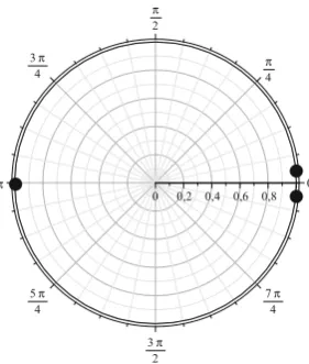
Fig. 3.4 Probability distribution after 100 steps of a quantum walk with the Hadamard coin starting from the initial conditionj .0/i D j0ijnD0i. The points where the probability is zero were excluded (nodd)
The third method is todownloadprogramQWalk1and follow the instructions on
how to choose the initial condition and the coin operator. A short description of this program can be found in Sect.5.2.5. This is the simplest method by far.
By employing any of the aforementioned methods the graph in Fig.3.4for the probability distribution after 100 steps will be obtained. Analogous to the classical random walk, we will ignore the null values of the probability. At t D 100, the probability is zero for all odd values of n. The asymmetry of the probability distribution is evident. The probability of finding the particle on the right side of the origin is larger than on the left. In particular, fornaround100=p2, the probability is much higher than at the origin. This fact is not exclusive to the valuet D 100. It is valid for any value oft. This suggests aballisticbehavior of the quantum walk. The particle can be found away from the origin as if it were in a uniform motion rightward. It is natural to ask whether this pattern would be held if the distribution were symmetric around the origin.
In order to obtain a symmetrical distribution, one must understand why the previous example has a tendency to go rightward. The Hadamard coin introduces a negative sign when applied to statej1i. This means there are more cancelations of terms with coin state equalsj1ithan of terms with coin state equalsj0i. Since the coin statej0iinduces movement rightward andj1ileftward, the final effect is the asymmetry with large probabilities on the right. We can confirm this analysis by calculating the resulting probability distribution when the initial condition is
j .0/i D j1ijnD0i:
Fig. 3.5 Probability distribution after 100 steps of a quantum walk with the Hadamard coin starting from the initial condition (3.23)
In this case, the number of negative terms will be greater than positive terms and there will be more cancelations of terms with the coin state inj0i. The final result will be the mirror distribution in Fig. 3.4 around the vertical axis. To obtain a symmetrical distribution, one must superpose the quantum walks resulting from these two initial conditions. This superposition should not cancel terms before the calculation of the probability distribution. The trick is to multiply the imaginary complex numberito the second initial condition and add to the first initial condition, as follows:
j .0/i D j0i pij1i
2 jnD0i: (3.23)
The entries of the Hadamard coin are real numbers. When we apply the evolution operator, terms with the imaginary unit are not converted into terms without the imaginary unit and vice versa. There will be no cancelations of terms of the walk that goes rightward with the terms of the walk that goes leftward. At the end, the probability distributions are added. In fact, the result is the graph in Fig.3.5.
If the probability distribution of the quantum walk is symmetric, the expected value of the position will be zero,i.e.hni D0:The question now is how the standard deviation .t /behaves as a function of time. The formula for the standard deviation of the probability distribution is
.t /D v u u t X1
nD1
n2p.t; n/; (3.24)
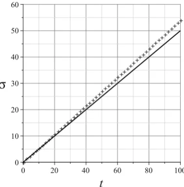
Fig. 3.6 Standard deviation of the quantum walk (crosses) and the classical random walk (circles) against the number of steps
performed in another chapter. For now, we will numerically calculate the sum of (3.24) by employing some computational implementation. The graphs in Fig. 3.6
show the standard deviation as a function of time for both the quantum walk (cross-shaped points) and classical random walk (circle-(cross-shaped points). In the classical case, we have .t / D pt. In the quantum case, we obtain a line, the slope being around 0.54,i.e. .t /D0:54 t
The linear dependence of the position standard deviation against time is an impressive result. Consider the following extreme situation: Suppose the particle has a probability of exactly one to go rightward. Aftert steps, it will certainly be found in the positionn D t. This movement is calledballistic. It is the motion of a free particle with unit velocity. The standard deviation in this case is obtained by replacingp.t; n/ byıt n in (3.24). The result is .t / D t. The quantum walk is ballistic, but the scape velocity is almost half of the free particle velocity. However, the quantum particle can be randomly found on the right or on the left side of the origin after measurement, which is a characteristic of random walks. The quantum probability distribution is spread in the intervalt =p2; t =p2, while the classical distribution is a Gaussian centered at the origin.
3.3
Classical Markov Chains
The discrete-time quantum walk model is not the only way toquantize classical random walks. We will describe a new quantum walk model that does not use a coin to determine the direction to move. Thecontinuous-time Markov chainsserved as the inspiration for the quantization that generated this new model.
When time is a continuous variable, the walker can go from vertexxj to an adjacent vertexxi at any time. One way to visualize the problem is to think of probability as if it were a liquid seeping from xj to xi. In the beginning, the walker is likely to be found inxj. As time goes by, the probability of being found in one of the neighboring vertices increases and the probability of staying in xj decreases. We have a transition rate which we denote by, assumably constant for all vertices (homogeneity and isotropy) and for all times. Therefore, the transition between neighboring vertices occurs with a probabilityper unit time. To address problems with continuous variables, we generally use aninfinitesimaltime interval, set up the differential equation of the problem, and solve the equation. If we take an infinitesimal time interval, the probability of the walker going from vertexxj to xi will be . Letdj be the degree of the vertexxj. Vertexxj hasdj neighboring vertices. It follows that the probability of the walker being in one of the neighboring vertices after timeisdj . Therefore, the probability of staying inxj is1dj . In the continuous case, the entryMij.t /of the transition matrix at timetis defined as the probability of the particle, which is in vertexxj, going to the vertexxi in the time intervalt. So
Mij./D
1dj CO.2/; ifiDj;
CO.2/; ifi ¤j. (3.25) Let us define an auxiliary matrix, calledgenerating matrixgiven by
Hij D 8 < :
dj;ifiDj;
; ifi¤j and adjacent; 0; ifi¤j and non-adjacent.
(3.26)
If we play a dice twice, the probability of getting six both times is the product of the probability of each move, as the moves are independent events. The same occurs in a Markov chain, because the next state of a Markov chain only depends on the current configuration of the chain. We can multiply the transition matrix at different times, so
Mij.tC/D X
k
Mi k.t /Mkj./: (3.27)
By isolating the termkDj and using the (3.25) and (3.26), we obtain Mij.tC/DMij.t /Mjj./C
X
k¤j
Mi k.t /Mkj./
DMij.t /.1Hjj/ X
k¤j
Mi k.t /Hkj:
By moving the first term on the right-hand side to the left-hand side and dividing it by, we obtain
dMij.t / dt D
X
k
HkjMi k.t /: (3.28)
The solution of this differential equation with initial conditionMij.0/Dıij is
M.t /DeH t: (3.29)
The verification is simple, if we expand the exponential function inTaylor series. With the transition matrix in hand, we can obtain the probability distribution at timet. If the initial distribution isp.0/E , we have
E
p.t /DM.t /p.0/:E (3.30)
It is interesting to compare this form of evolution of the continuous-time Markov chain with discrete-time chain, given by (3.10).
Exercise 3.9. Show that the uniform vector is an eigenvector ofH with eigen-value 0. Use this fact to show that the uniform vector is the eigenvector ofM.t / with eigenvalue 1. Show thatM.t /is a stochastic matrix for allt 2R.
Exercise 3.10. What is the relationship betweenHand the Laplacian matrix of the graph?
Exercise 3.11. Show that the probability distribution satisfies the following differ-ential equation:
dpi.t / dt D
X
k
Hkipk.t /:
3.4
Continuous-Time Quantum Walks
with the coin and the Hilbert space associated with the shift operator, which was accomplished with the tensor product, according to the postulates of Quantum Mechanics.
In the passage from thecontinuous-time Markov chainsmodel to the continuous-time quantum walkmodel, again we use a quantization process in this new context. Note that the continuous-time Markov chain has no coin associated. Therefore, we simply convert the vector that describes the probability distribution to a state vector and the transition matrix to an equivalent unitary operator. We must pay attention to the following detail: matrixH, given by (3.26) is Hermitian, so matrixM given by (3.29) is not unitary. There is a very s