Exploratory Policy Research: An Application
to the Assessment of Regional Tourist Multipliers
Sef Baaijens and Peter Nijkamp, Department of Economics, Free University Amsterdam
This article addresses the question how meta-analytic methods can be used to draw quantitative economic inferences on case studies (or phenomena) when actual information is scarce. It argues that the recently developed rough set theory may offer an operational contribution to impact assessment on the basis of transferability of research findings from previous case study research findings on similar phenomena. This approach is able to identify band widths of plausible outcomes in light of prior knowledge. This new analysis framework is illustrated by means of an empirical investigation into the size of tourist income multipliers in various tourist areas, with a particular focus on the Greek island Lesvos. 2001 Society for Policy Modeling. Published by Elsevier Science Inc.
1. TRANSFERABILITY OF SCIENTIFIC RESULTS
Empirical policy research is often faced with the challenge to produce meaningful results in a limited time span. In many cases there is no possibility for thorough field work or original statistical or econometric experiments. At best lessons may then be drawn from comparable quantitative studies undertaken elsewhere. This provokes the methodological question on transferability of re-search findings.
Scientific knowledge acquisition is ideally a continuing process of hypothesis formulation, derivation of propositions, data collec-tion, empirical testing, and revision of hypotheses. Especially in ex-perimental sciences (e.g., medicine, chemistry, psychology) where
Address correspondence to P. Nijkamp, Department of Economics, Free University, De Boelelaan 1105, 1081 HV Amsterdam, The Netherlands.
Received March 1997; final draft accepted December 1997. Journal of Policy Modeling22(7):821–858 (2000)
background conditions can often be controlled, this methodologi-cal approach has created a formidable advance in scientific in-sights. In nonexperimental applied social science research, how-ever, we are usually confronted with only partly—or at best largely—similar phenomena, mainly because relevant background conditions may significantly differ. In such cases, the question arises as to whether the methodological chain described above is still meaningful in obtaining generalizable or transferable research findings. Besides, if a given distinct phenomenon or object of study is investigated with the help of varying new background data, it may very well happen that through (partial) overlap or correlation redundant information is used. The marginal scientific benefits of additional studies on largely similar phenomena tend to decline, when the most interesting facts are already known from previous studies. In this context, it is an intriguing question in how far and under which conditions transferability of results from comparable studies can be postulated. Clearly, in case of controlled experi-ments (with equal background factors and a clear dichotomy be-tween the objects investigated), this endeavor is a relatively easy task. But in the large majority of social science studies, we do not have controlled experiments with homogeneous measurement scales, but rather fragmented results from various studies that focus on similar issues, but are usually heterogeneous in nature. More heterogeneity usually means less transferability of results, unless this is compensated by a large sample of experiments or objects. Do however, more studies lead to better insights? This fascinating methodological question will be dealt with in this paper by investi-gating the potential ofmeta-analysisas a methodological tool for transferability of research results in the applied social sciences.
as a methodological tool for comparative study in the social sci-ences. Examples can be found in psychology, labor economics, environmental science, and transportation science (see, among others, Fiske, 1983; Mitra, Jenkins, and Gupta, 1992; Button, 1995; Smith, 1995). However, in many cases the sample of applied case studies on a given phenomenon is rather small (say, 10 to 15), and then the intriguing question arises whether there is still meaningful scope for meta-analytical approaches. This means that statistical (probabilistic) methods are less appropriate. The main aim of the present paper is to demonstrate that an approach based on the recently developed multidimensional classification method, coined
rough-set analysis, may then be very suitable, as this method is able to deal with pattern recognition in categorical variables and to derive logical binary statements from a given data set. This method will also empirically be demonstrated in this paper by means of an analysis of tourist income multiplier values from various modeling studies on tourist areas all over the world.
In light of these remarks, the paper is organized as follows. Section 2 will be devoted to a concise presentation and critical discussion of meta-analysis. Then, in Section 3, we will propose the use of rough-set methods for categorical information, especially in situations of a small number of case studies; the main principles of the rough-set methods will also be described. We will then illustrate in subsequent sections the usefulness of rough-set analy-sis as a methodological tool for meta-analyanaly-sis by presenting and comparing various results from previous studies on the assessment of tourist income multipliers. In addition to a comparative analysis, we will also try to approximate the value of a tourist multiplier for a case where no field information but only information on background variables is available, viz. the Greek island of Lesvos. Finally, we will offer some reflective conclusions.
2. META-ANALYSIS IN THE SOCIAL SCIENCES
1994; Button and Nijkamp, 1996). The meta-analytic approach comprises the systematic application of a range of quantitative methods to assess common characteristics and variations across a set of actually separate, but largely similar case studies on more or less the same type of phenomenon. A major advantage of meta-analysis is its ability to create scientific consensus on the underlying variation in findings from individual case studies, as the results have to be based on solid analytical methods.
In general terms, the meta-analytical approach provides a series of techniques that allow the cumulative results of a set of individual studies to be pulled together. It permits a quantitative aggregation of results across comparable studies. In this way it does not only provide more accurate evaluations of quantitative parameters, but it may also offer new insights into phenomena for which as yet no specific study exists. It may also help to pinpoint judgement bias and to provide more clearly defined inferences on the eco-nomic costs and benefits from the plethora of data that exists. It may act as a supplement to more common literary type of analyti-cal approaches when reviewing the usefulness of parameters de-rived from prior studies and help direct new research to areas where there is a clear need for generalization and transferability. A good description of the potential of meta-analysis can be found in Cook et al. (1992): “Meta-analysis offers a set of quantita-tive techniques that permit synthesizing results of many types of research, including opinion surveys, correlational studies, experi-mental and quasi-experiexperi-mental studies and regression analysis probing causal models. In meta-analysis the investigator gathers together all the studies relevant to an issue and then constructs at least one indicator of the relationship under investigation from each of the studies. These study-level indicators are then used (much as observations from individual respondents are used in individual surveys, correlational studies, or experiments) to compute means, standard deviations and more complex statistics.” In conclu-sion, meta-analysis seeks to gain additional scientific insights in a variety of ways from previous investigations. These ways are:
(1) combining and averaging, possibly using weights, estimated values, or basic relationships, performance indicators or achievements;
(3) aggregating studies, by considering complementary results or explanations;
(4) apprehending common elements in different studies of a similar phenomenon;
(5) evaluating different methods applied to similar questions or research issues; and
(6) tracing key factors that are responsible for differing results across similar studies or research endeavors undertaken elsewhere.
Traditional meta-analytic techniques were often based on quali-tative literature reviews and had several intrinsic limitations, so that the interpretation of results should be undertaken with great caution. The following caveats regarding such conventional meta-analytic approaches ought to be mentioned: (1) The output of most traditionally conducted reviews tends to be only in the form of taxonomies of findings, without any specific attempt to relate these to the intrinsic review purpose or the underlying methodol-ogy. (2) Subjectivity tends to accompany usually a basically literary type approach to synthesizing scientific results (Button, 1994). The convictions and opinions following from literature reviews done by leading scientists often had much value attached to them, not always in the least because of their scientific status. But it ought to be recognized that narratively reviewing literature gives more room for subjective interpretations than does a statistical analysis. (3) Traditional literary reviewing may be scientifically unsound, unless it embraces sound statistical practice. A common problem is that if a majority of studies come up with similar conclusions, these are accepted on an implicit voting basis, irrespective of the quality of the data or reliability of the techniques employed. (4) A traditional review process may also be less appropriate because of the difficulties of mentally handling a large number of different findings. So the fundamental problem with narrative reviewing techniques are the mind’s limitations and the magnitude of the task to which it is applied.
has frequently, though not exclusively, been concerned with mod-eratorvariables by seeking for commonalities in background vari-ables Most of the work that has been conducted in this field has employed meta-regression analysis of the general form (Stanley and Jarrell, 1989):
Yj5 b 1 SakZjk1uj(j51,2, . . .J) (k51,2, . . .K), (1)
whereYjis the reported estimate of the variable of interest in the
jth study from a total of J studies; b is an intercept (e.g., the summary value of Y); Zjk are variables that reflect the relevant
characteristics of an empirical study that could explain variations amongst various studies;akare the coefficients of theKdifferent
study characteristics which are controlled for; and finally,ujis the
error term.
This methodology is based on conventional statistical methods
that have the advantage that they are well understood by social scientists and have been extensively used in meta-analysis work in the natural sciences. These techniques can play useful roles in quantitative comparative studies (e.g., Cook and Leviton, 1980; Hunter et al., 1982; Light and Pillemer, 1984; Hedges and Olkin, 1985; Wolfe, 1986; Wachter, 1988; Mann, 1990; Rosenthal, 1991; Button, 1994). The problem is that they require information to be presented in a manner that is amenable to statistical analysis, and this may limit both the range of topics that can be treated or the types of effect that can be considered across a range of studies. Discrete modeling procedures have, in recent years, reduced this limitation, but the restricted scope still remains for small samples. Next to this standard statistical approach, there are also various forms ofmeta-multicriteria analysis, ranging from simple frequency countings to multidimensional trade-offs. These can be very useful for evaluation purposes, especially where multiple criteria, or ob-jectives, may underlie a comparison of different, but similar stud-ies. This is especially relevant when studies do not offer a simple estimation of an important indicator or where the interest lies in looking at a number of performance indicators (see Greco, Matarazzo, and Slowinski, 1995).
offering a robust system of notations for expressing and communi-cating uncertainty in quantitative information. When either sys-tem’s uncertainties or decision stakes are large, a new approach is required in judging, evaluating, or summarizing existing insights. The authors make a plea for an “extended peer community,” which is to involve all stake-holders related to the respective situation or issue, including citizens, experts, and policy makers. It should allow for a multidimensional, multiperspective approach, which explicitly treats the emergent complexity of systems. It allows meta-analysis to deal with policy studies that are not limited to unidimensional estimates of a given variable, but cover a whole range of issues of a qualitative and complex nature, including trade-off and distributional issues.
Finally, there is rough-set analysis, which is a nonparametric method that is able to handle a rather diverse and less immediately tangible set of factors. Rough-set analysis, proposed in the early 1980s by Pawlak (1982, 1991), provides a formal tool for trans-forming a data set, such as a collection of past examples or a record of experience, into structured knowledge, in the sense of ability to classify objects in distinct classes of attributes (Van den Bergh, Matarazzo, and Munda, 1995; Matarazzo, 1996). In such an approach it is not always possible to distinguish objects on the basis of given information (descriptors) about them. This imper-fect information causes indiscernibility of objects through the val-ues of the attributes describing them. The rough-set theory has proven to be a useful tool for large class of qualitative of fuzzy multiattribute decision problems. It can effectively deal with prob-lems of explanation and prescription of a decision situation where knowledge is imperfect. It is helpful in evaluating the importance of particular attributes and eliminating redundant ones from a decision table, and it may generate sorting and choice rules using only the remaining attributes so as to identify new choice options in policy problems and next to rank them. Further details of rough set analysis can be found in Section 3.
A very interesting, essentially meta-analytic comparative re-search endeavor on differences in economic development in vari-ous countries can be found in Morris and Adelman (1988). The authors used an extensive data set (socio-economic indicators on groups of countries) in order to identify—by means of disjoint principal components methods—the importance of institutional patterns and changes therein for the course of development of these countries.
Meta-analysis can thus be a powerful analytical tool in compara-tive studies, but its limitations would have to be recognized. Ele-mentary mistakes are made when a variety of study outcomes is treated with procedures invented for a statistical sample of experimental outcomes without the benefit of (1) controlled condi-tions, (2) homogeneous measurement scales, and (3) statistical independence, that makes the procedure valid (Wachter, 1988). It should also be noted that a proper meta-analysis would, theoreti-cally, require looking at all relevant studies done in the field, also the unpublished ones. (The Economist, 1991); especially negative results tend to be left out in official publications. Furthermore, there is no guarantee that the original studies in a meta-analytic approach are not biased (The Economist, 1991), so that we face the question whether one should include all studies done in the field or otherwise specify criteria for selection in advance. Ideally, there must be an existing body of studies which can be subjected to statistical procedures in the broadest meaning of the term. The number of studies need not be large (e.g., some medical meta-analyses have involved as few as three studies), but ideally it should not be too small; normal statistical criteria favor the use of as many observations as possible.
There must also be a degree of commonality in the prior infor-mation to be examined. This may, for example, be spatial, temporal or subject specific, but without this the realm of analysis would be excessively diverse. Defining the extent of commonality is itself a potential problem and is inevitably subjective. In some cases the problem of diversity may be contained, if it is possible to isolate the peculiarities of studies and to normalize them in the meta-analysis itself.
categorical, qualitative, fuzzy). In recent years, rough set theory has emerged as a powerful analytical tool for dealing with “soft” data. The rough-set theory aims to offer a classification of data measured on any information level by manipulating data in such a way that a range of consistent and feasible cause–effect relation-ships can be identified, while it is also able to eliminate redundant information. Section 3 will offer a concise description fo the main principles of the rough set theory.
3. ROUGH SET ANALYSIS AS A META-ANALYTIC SOFT MODELING TOOL
In the framework of our meta-analytical approach, we will show that rough-set analysis can be a very useful tool in case of imprecise or qualitative information. Therefore, we will give a concise intro-duction to rough set theory (see also, Pawlak, 1991; Slowinski, 1993; Greco et al., 1995; Matarazzo and Nijkamp, 1995; Matarrazo, 1996). A rough set is characterized by the fact that it is uncertain in advance which objects belong precisely to that set, although it is in principle possible to identify all objects that may belong to the set at hand. The rough-set theory takes for granted the existence of a finite set of objects for which some information is known in terms of factual (qualitative or numerical) knowledge on a class of attributes (features, characteristics). These attributes may also act asequivalence relationships for these objects, so that an ob-server can classify objects into distinct equivalence classes. Objects in the same equivalence class are—on the basis of these features concerned—indiscernible.In case of multiple attributes, each attri-bute is associated with a different equivalence relationship. The intersection of multiple equivalence relationships is called the indiscernibility relationship, with respect to the attributes con-cerned. This intersection generates a family of equivalence classes that is a more precise classification of the objects than that based on a single-equivalence relationship. The family of equivalence classes that is generated by the intersection of all equivalence relationships is called the family of elementary sets. The classifica-tion of objects as given by the elementary sets is the most precise classification possible, on the basis of the available information.
other words, a set is rough if it is not equal to a union of elementary sets. In this framework, two new concepts are introduced, viz. the
lower and upper approximation in order to identify a range of uncertainty for the assignment of objects. The lower approxima-tion of a setYis the union of all elementary sets that are a subset of Y. The upper approximation of a set Y is the union of all elementary sets that have a nonempty intersection withY.
This approach leads thus to an imprecise representation of real-ity due to the “granularreal-ity” of knowledge; in other words, realreal-ity is represented by “granules,” corresponding to the elementary sets, i.e., subsets of the universe whose elements are indiscernible (indistinguishable) by the set of attributes used, because they present the same description in terms of the values of these attri-butes. The “granularity” of knowledge representation is used to define the key concepts of the rough-set theory. The size of these “granules” depends, naturally, on both the number of attributes used for the description of the objects and the domain of each attribute. With a suitable variation in these two quantities it is possible to obtain a variation in the dimensions of the “granules;” an increase in the number of attributes and in the number of values that each attribute can assume, results in more “granules.” Next, lower and upper approximations can be determined on the basis of the typology (“granules”) generated by the available information on the elements of the relevant set (indiscernibility relation), that is, on the ability to observe some real phenomena (objects), classify them, distinguish them on the basis of the infor-mation obtained from real-world observations, or of prior knowledge from an expert. The representation of reality by means of the rough sets is, therefore, based on the knowledge (objective or subjective) on reality and the capacity to classify the information obtained.
Now we may introduce the concept of a reduct. A reduct is a subset of the set of all attributes with the following characteristic: adding another attribute to a reduct does not lead to a more accurate classification of objects (i.e, more granules), while elimi-nation of an attribute from a reduct does lead to a less accurate classification of objects (i.e., less granules).
Based on the previous concepts, the rough-set theory is now able to specify various decision rules of an “if then” nature. For specifying decision rules, it is useful to represent our prior knowl-edge on reality by means of an information table. An information table is a matrix (objects rowwise, attributes columnwise) that contains the values of the attributes of all objects. In an informa-tion table the attributes may be partiinforma-tioned intocondition (back-ground) and decision (response) attributes. A decision rule is then an implication relationship between the description of the condition attributes and that of a decision attribute. Such a rule may be exact or approximate. A rule is exact if the combination of the values of the condition attributes in that rule implies only one single combination of the values of the decision attributes, while an approximate rule only states that more than one combina-tion of values of the decision attributes correspond to the same values of the condition attributes. Decision rules may, thus, be expressed as conditional statements (“if then”).
In this way one may analyze in greater depth the information contained in the original table and to enrich it, specifying addi-tional decision rules directly by means of suitable interviews or discussions with experts. In other words, it is also possible to acquire information directly in the form of decision rules supplied by experts, thereby enriching the original information contained in the decision table.
In practice, therefore, it is possible to use both the decision rules obtained by elaborating the data contained in the decision table and, if necessary, further rules supplied and suggested by experts. The former may be accompanied by an indicator of their “strength,” for example, the frequency (absolute or relative) of events in agreement with each decision rule. Moreover, both the former and the latter may be based on suitable and different sets of condition attributes, containing a larger or smaller number of attributes (even a single attribute) This last case implies that the value assumed by an attribute is sufficient to guarantee that the decision attribute (or attributes) will assume certain values, what-ever the values of the other condition attributes. This consider-ation assumes particular importance whenincomplete information
Decision rules, which constitute the most relevant aspects of the rough-set analysis, may be applied immediately in order to supply recommendations and advice in problems ofmultiattribute sorting, that is, in the assignment of each potential action to an appropriate predefined category according to particular aims. In this case, the classification of a new object may be usefully under-taken by a comparison between its description (values of the condition attributes) and the values contained in the decision rules. These are more general than the information contained in the original decision table, and permit a classification of new or additional objects in larger numbers and more easily than would be possible using a direct comparison between these and the original examples. In general, such decision rules allow to make conditional transferable inferences as the “if” conditions specify the initial conditions, while the “then” inference statements highlight the logical valid conclusions. In contrast to principal component analy-sis where initial quantitative data are grouped into new compound variables, rough-set analysis uses (both quantitative and qualita-tive) data to extract conditional (“causal”) statements on the likely occurrence of a given response variable. In this way, rough-set analysis can also be used as a tool for conditional transferability of results from some case study to a new situation. The mathemat-ics of the rough set is rather complicated, but has been properly described in the literature. We will now illustrate the relevance of rough-set analysis by applying it to a case study on comparative analysis of tourist income multipliers.
4. A META-ANALYTIC APPROACH TO TOURISM
As mentioned above, meta-analysis ma be conceived of as quasi-controlled laboratory experimentation with a limited sample of observations drawn under different conditions. Thus, the focus is on systematic variations in the estimated outcomes (or responses), by analyzing the nature of the explanatory variables, the informa-tion base (e.g., geographical scale, time periods, geographical loca-tion, etc.) and the statistical/econometric techniques used. In this way, the responsiveness of a compound system to various back-ground factors can be explored in a way that makes the results more transferable across varying situations, and even to situations where no directly measurable outcomes do exist.
relation to island economies. Tourism has become an important economic sector at a global scale (e.g., in Europe it represents some 5 percent of the national product), partly as a result of the rise in welfare (and the consequent rise of a leisure society and improvement in transport systems), and partly also as a result of environmental decay (or decline in quality of life) in countries of origin (Pearce, 1989). This has led to massive flows of tourism all over the world, in particular to typical tourist cities (e.g., Venice, Paris, Amsterdam, etc.) or to sites with a natural beauty (e.g., the Bahamas, Santorini, the Seychelles, etc.).
For most countries, the consequences of tourism are twofold (see Giaoutzi and Nijkamp, 1993). In the first place, tourism makes up a source of additional local or regional revenues to such an extent that it may even become a dominant economic sector (e.g., Crete, Hawaii). Secondly, the visual, cultural, or natural attrac-tiveness of a site may be affected or even destroyed by tourism, especially if it takes place at a large scale (e.g., coastal areas in Spain, Italy, or Florida) (Pearce and Turner, 1990). Here we are often witnessing the so-called tourism paradox (Coccossis and Nijkamp, 1995): tourism is a way of escaping from unfavorable living conditions in a country of origin to enjoy temporarily an attractive quality of life elsewhere; in doing so, a transfer of finan-cial resources is taking place to the country of destination, but in turn, the tourist flows also cause an erosion of the basis upon which tourism rests, viz. visual, cultural, or natural beauty.
Consequently, a country of destination is faced with a difficult trade-off, viz. additional income versus a decline in quality of life. It is thus of paramount importance to assess the direct and indirect revenues accruing from tourism in relation to environmental qual-ity conditions in the area concerned.
In the past decades, several studies have been carried out on the economic consequences of tourism. Most studies on the eco-nomics of tourism focus on the assessment of the multiplier effects of tourism in a holiday resort. Many of these studies are concerned with island economies, as islands are often attractive tourist places and as the economic consequences are relatively easier to map out in a more or less closed island system. There is, thus, a clear need for an assessment of relevant impacts (e.g., employment, income, environment, etc.) (see also, Pleeter, 1980; Nijkamp and Blaas, 1994). A central concept in tourism impact analysis is the
various types of expenditure; the average tourist income multiplier is then the ratio of total regional income generated by an average unit of tourist expenditure. In view of the increasing importance of the tourist sector in various areas, several studies have been carried out to estimate for a given site the order of magnitude of the tourist multiplier. If one makes a cross-sectional comparison of the various outcomes, one finds a range of different values of the tourist multiplier for such tourism economies. This observation is intriguing, and requires a closer investigation. A first method may be to undertake a qualitative literature research to identify significant differences in background variables, but it seems more plausible to resort to meta-analytical techniques to obtain a more solid basis for statistical inference.
In the context of our study, we will go one step further. In addition to an explanation of differences in quantitative results under varying conditions, we will also try to predict (a range of values of) multiplier values of a tourist economy in a situation where we only have insight into the background variables. Thus, we will use meta-analytical methods as a tool for transferability of quantitative outcomes (responses) in different situations. This exercise may have great practical relevance, as it would avoid designing and undertaking painstaking and laborious field surveys that are otherwise necessary to estimate a regional input–output model. We will apply our analysis to the Greek island of Lesvos.
5. MULTIPLE MULTIPLIERS
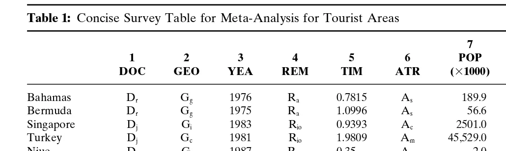
The start of a meta-analytical exercise is to collect documented studies on income multiplier effects of tourist areas, notably re-gional economies. We were able to identify a sample of 11 relevant and officially published case studies on tourist regions from differ-ent sources and covering differdiffer-ent years (see Table 1) The informa-tion provided by the study reports serves as the principal data base in the meta-analysis. Clearly, not all relevant data were directly available for a comparative quantitative analysis, as several data were more or less hidden in the study reports. Therefore, a system-atic inventory of all relevant information had to be made. This investigation was made with the help of a list of relevant topics (see Appendix 1), by making also use of a general framework of economic meta-analysis as described by Button (1995). A closer investigation of the study reports led to a systematic overview of the relevant information contained in these reports. This overview, however, appeared to be far from complete, as each individual study contained differences in approach and viewpoint, so that the similarity in the information provided left much to be desired. As a consequence, the meta-analysis was restricted to information that was commonly known for most geographical areas considered. The final selection of the cross-sectional case-study features is contained in Table 1. Ideally, one would wish to have more specific economic variables, such as the value-added ratio or the import ratio, or more specific tourist information such as tourist days or purchasing power parity data. Unfortunately, these data were not available to a sufficient extent in the study reports to warrant a solid meta-analysis. Clearly, missing information limits the use of cross-sectional comparisons.
The range of variation in the multiplier values appears to be rather significant. Consequently, it does not make sense to make an average estimate of such a multiplier for any new case study. Rather, it is necessary to link the value of these multipliers to differences in background variables using meta-analytical tech-niques. This will be done in the next section.
6.1. A META-ANALYSIS OF TOURIST MULTIPLIERS 6.A. Introduction
S.
Baaijens
and
P.
Nijkamp
Table 1: Concise Survey Table for Meta-Analysis for Tourist Areas
7 8
1 2 3 4 5 6 POP SUR 9 10 11
DOC GEO YEA REM TIM ATR (31000) (31000) TOA LCS POA
Bahamas Dr Gg 1976 Ra 0.7815 As 189.9 11,401 1388.0 75.8 y
Bermuda Dr Gg 1975 Ra 1.0996 As 56.6 107 511.4 86.6 n
Singapore Dj Gi 1983 Rio 0.9393 Ac 2501.0 625 2856.6 ? y
Turkey Dj Gc 1981 Rio 1.9809 Am 45,529.0 779,425 1460.0 ? y
Niue Dj Gi 1987 Ra 0.35 An 2.0 258 1.8 78.0 n
Cook Islands Dj Gg 1984 Ra 0.43 As 18.0 236 25.6 40.0 n
Kiribati Dj Gg 1987 Ra 0.37 An 66.0 270 2.0 ? y
Tonga Dj Gg 1987 Ra 0.42 As 95.0 699 16.1 24.2 y
Vanuatu Dj Gg 1987 Ra 0.56 Am 140.0 12,200 17.5 52.0 y
Alonnisos Db Gi 1989 Rio 0.489 As 1.55 83 20.0 35.9 n
Okanagan Dj Gr 1977 Rio 0.713 An ? 21,813 1400.0 ? n
1. Type of documentation (DOC): Dr: research paper; Dj: journal; Db: book.
2. Geographic feature of the area (GEO): Gs: single island; Gg: island group; Gr: region; Gc: country. 3. Year of collection of data (YEA).
4. Research method (REM): Rio: input–output model; Ra: Archer method. 5. Estimated value of the average tourist income multiplier (TIM).
6. Type of tourist attractiveness (ATR): As: sun; Ac: culture; An: nature; Am: mixed. 7. Population size (POP).
8. Surface (in km2) (SUR). 9. Tourist arrivals (TOA).
with the medical experimentation model. In the medical model the definition of control groups is unambiguous, the estimation of impact parameters is based on a probability model, and the impact assessment boils down to a probability statement in terms of the chance that the effect belongs to a given impact interval. In our case of 11 tourist studies, we do not have a controlled experiment on sampling among households, tourists, and other economic sectors in the regional economy (the studies are given). Furthermore, the tourist analysis is carried out on a meso level of aggregation, and finally, in these studies the (questionable) assumption is made that the measured (or estimated) multiplier (via the input–output of the Archer model) is also the real one and not subject to stochasticity (see, for details, Baaijens, 1996). Our meta-analytical approach to the comparison and assess-ment of tourist income multipliers will be based on two stages, viz. a linear regression model on the moderator variables of the multipliers and rough-set analysis of the background variables with respect to the tourist income multipliers. The results will now successively be presented and discussed.
6.B. Linear Regression of the Moderator Variables
value. The hypothesis is, therefore, that there is a positive relation-ship between the degree of economic diversity and the multiplier. Because there is not a uniform measure for economic diversity, we use the indicators population size and area size to test this hypothesis. This boils down to the hypothesis that there are posi-tive relationships between the multiplier and population size, and between the multiplier and the size of the area. In addition, it seems also plausible that politically independent areas have a relatively higher multiplier value due to a higher degree of import substitution than nonindependent regions. (2) A meta model, where the typical meta variables are included in the explanatory analysis, for example, the source of the study, the year of collection of data, the analysis method used. Meta variables refer to method-ological choices made in the original studies; their values are largely independent from the object of study in the meta-analysis. In this case, dummy variables may be introduced. A plausible hypothesis is that the input–output model will generate higher multiplier values than the Archer model, as the first one addresses system-wide economic effects more thoroughly. (3) A tourist model, where the size of the multiplier will be linked to incoming tourist flows. It seems plausible to assume that there is a positive correlation between the size of the tourist flow and the multiplier effect. A tourist area that receives a relatively large number of tourists in comparison to the number of inhabitants, is however, expected to have a relatively low multiplier. The idea is that the tourist sector will crowd out other sectors in case of too many tourists (with respect to labor and capital). As a consequence, the economic diversity in the region will decline, which leads to lower multiplier values.
Clearly, these hypotheses can only partly and provisionally be tested because of our limited sample.
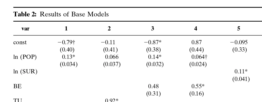
Base model:in the base model a series of experimental regres-sion analyses on the base variables is carried out. The most impor-tant results are contained in Table 2. Due to the small sample, only indicative conclusions can be drawn.
METHODS
FOR
P
OLICY
RESEARCH
839
Table 2: Results of Base Models
var 1 2 3 4 5 6 7 8
const 20.79† 20.11 20.87* 0.87 20.095 0.49 21.29* 20.75
(0.40) (0.41) (0.38) (0.44) (0.33) (0.31) (0.31) (0.39)
ln (POP) 0.13* 0.066 0.14* 0.064† 0.21* 0.15*
(0.034) (0.037) (0.032) (0.024) (0.032) (0.043)
ln (SUR) 0.11* 0.019
(0.041) (0.044)
BE 0.48 0.55*
(0.31) (0.16)
TU 0.92* 1.24* 0.56
(0.36) (0.41) (0.30)
GEO 21.00*
(0.23)
POA 20.64* 20.48*
(0.19) (0.19)
R2 0.66 0.82 0.75 0.94 0.45 0.59 0.87 0.92
n 10 10 10 10 11 11 10 10
Note:standard deviations are given in parentheses.
* The null hypothesis that this coefficient is zero is rejected at a significance level of 5 percent.
† The null hypothesis that this coefficient is zero is not rejected at a significance level of 5 percent, but is rejected at a significance level of 10 percent.
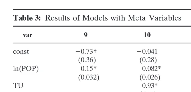
Table 3: Results of Models with Meta Variables
var 9 10 11 12
const 20.73† 20.041 20.41 0.0025
(0.36) (0.28) (0.51) (0.47)
ln(POP) 0.15* 0.082* 0.12* 0.064
(0.032) (0.026) (0.037) (0.039)
TU 0.93* 0.84†
(0.25) (0.40)
DOC 20.35 20.36*
(0.20) (0.12)
REM 20.28 20.12
(0.23) (0.20)
R2 0.76 0.93 0.71 0.83
n 10 10 10 10
Note:DOC51 if the documentation type is a journal article, 0 otherwise; REM51 if the TIM has been calculated with the model of Archer, 0 if the TIM has been calculated with an input–output model.
* The null hypothesis that this coefficient is zero is rejected at a significance level of 5 percent.
† The null hypothesis that this coefficient is zero is not rejected at a significance level of 5 percent, but is rejected at a significance level of 10 percent.
Next, also the size of the area has been investigated. The regres-sion results appear to support the hypothesis that regions with a larger surface have a higher tourist multiplier. Because, again, Turkey appears to have a larger residual, a dummy variable has been included for this area. In that case, the result becomes far less significant, so that a positive relationship between surface and the tourist multiplier is not plausible.
Finally, the impact of the degree of political autonomy has also been examined. In contrast to our hypothesis, we find a significant negative relationship between the income multiplier and political autonomy.
Meta model:the meta model has been experimented in combina-tion with he most significant variable from the base model, i.e., population size. The results can be found in Table 3.
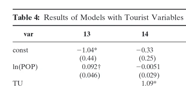
Table 4: Results of Models with Tourist Variables
var 13 14 15 16
const 21.04* 20.33 21.25* 20.57
(0.44) (0.25) (0.41) (0.32)
ln(POP) 0.092† 20.0051 0.16* 0.096*
(0.046) (0.029) (0.031) (0.027)
TU 1.09* 0.86*
(0.22) (0.24)
ln(TOA) 0.066 0.092*
(0.052) (0.025)
TI 0.043† 0.039*
(0.021) (0.013)
R2 0.64 0.95 0.79 0.93
n 10 10 10 10
Note:TOA5number of tourist arrivals in the year of investigation; TI5tourist index: the ratio of the number of arrivals (TOA) to the population size (POP).
* The null hypothesis that this coefficient is zero is rejected at a significance level of 5 percent.
† The null hypothesis that this coefficient is zero is not rejected at a significance level of 5 percent, but is rejected at a significance level of 10 percent.
appear to be lower than those published elsewhere: there is appar-ently, on average, a tendency towards some overestimation in less official publication channels.
Next, it is also noteworthy that the type of model used has an impact on the results: the Archer model tends to yield, on average, lower values of the tourist income multiplier than the input–output model.
Tourist model: in the final stage we will investigate the impact of tourism-specific variables, in addition to the previous significant variables of population size and Turkey (dummy). The results are contained in Table 4. There is some indication that higher tourist arrivals lead to a higher multiplier value, but there are interfering effects from the dummy variable for Turkey. The impact of the tourist index (ratio of incoming tourists to population size), how-ever, appears to be positive.
the next subsection we will deal with results obtained by rough-set analysis.
6.C. A Rough Set Analysis
As mentioned above, the rough-set theory is essentially a classi-fication method, devised for nonstochastic information. This also means that ordinal or categorical information (including dummies) may be taken into consideration. This makes rough-set analysis particularly useful as a meta-analytical tool in case of incomplete, imprecise, or fuzzy information.
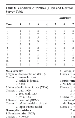
The implementation of a meta-analysis of the tourist income multiplier by means of rough set analysis proceeds in three succes-sive steps. The first step is to choose the information (the study characteristics) that will be analyzed. We have chosen for the information contained in the survey table from Section 5 (see Table 1). This table contains the information that is known for almost all tourist areas considered. The second step is the classifi-cation of this original information. All objects (in this case, tourist areas) are classified into various categories for each attribute sepa-rately. This applies to both categorical and ratio information. In general, some sensitivity analysis on the classification used is meaningful, as a balance has to be found between homogeneity and class size. The classification exercise leads to a coded informa-tion table, in which all objects (tourist areas) are subdivided into distinct classes for each attribute. The third step is the investigation of the coded information table by means of rough set analysis, by calculating reducts of attributes and applying minimal decision algorithms (as outlined above).
Table 5: Condition Attributes (1–10) and Decision Attribute (d) from
Meta variables 6 Political autonomy (POA)
1 Type of documentation (DOC) Classes: 1 independent (I) Classes: 1 research paper 2 not independent (NI)
2 article in journal Tourist variables
3 book 7 Number of tourist arrivals (TOA) 2 Year of collection of data (YEA) Classes: 1 <10,000 (S)
Classes: 1 until 1979 2 10,000–700,000 (M) 2 1980 until 1985 3 .700,000 (L)
3 from 1986 8 Share of arrivals from most important 9 Research method (REM) country of origin in total number of arriv-Classes: 1ad hocmodel of Archer als “largest country share” (LCS)
2 input-output model Classes: 1 <45% (S)
Geographic variables 2 45–75% (M)
3 Population size (POP) 3 .75% (L)
Classes: 1,10,000 4 no available information 2 10,000–100,000 10 Type of tourist attractiveness (ATR) 3 100,000–200,000 Classes: 1 “sun, sand and beach holidays” 4 200,000–1,000,000 2 nature and culture holidays 5 1,000,000–5,000,000 (NC)
6 .5,000,000 3 “mixed,” i.e. both “sun, sand 7 no available information and beach holidays” and nature 4 Surface (in km2) (SUR) and culture holidays (MI)
Classes: 1<500 (VS5very small) Decision variable
2 500–10,000 (S5small) d Average tourist income multiplier (TIM) 3 10,000–100,000 (M5 Classes: 1 <0.5 (S)
medium) 2 0.5–1.0 (M)
4 .100,000 (L5large) 3 1.0–1.5 (L)
5 Geographic feature of the area (GEO) 4 .1.5 (VL5very large) Classes: 1 island
2 archipel
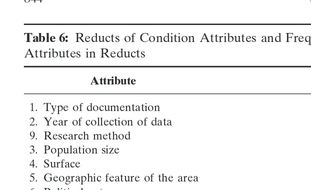
Table 6: Reducts of Condition Attributes and Frequency of Attributes in Reducts
Attribute Frequency (%)
1. Type of documentation 9 (42.9%)
2. Year of collection of data 4 (19.0%)
9. Research method 3 (14.3%)
3. Population size 211 (14.3%)
4. Surface 612 (38.1%)
5. Geographic feature of the area 213 (23.8%)
6. Political autonomy 411 (23.8%)
7. Number of tourist arrivals 313 (28.6%)
8. Largest country share 217 (42.9%)
10. Type of tourist attractiveness 712 (42.9%) Reducts of condition attributes:
with meta variables: {2,7,10}, {1,7,10}, {2,6,10}, {1,4,10}, {2,4}, {1,5,6,10}, {1,6,9,10}, {1,3}, {2,3}, {1,4,9}, {1,4,8}, {1,4,7}, {1,4,5}, {6,8,9,10}
without meta variables: {3,8}, {7,8,10}, {4,8,10}, {5,6,8}, {5,7,8}, {4,7,8}, {4,5,8}
Note:For other variables than meta variables, Table 6 indicates first the frequency of their occurrence in reducts with meta variables and second, the frequency of their occur-rence in reducts without meta variables.
This method has been implemented in a computer program by Slowinski and Stefanowski (1992). This software was used here to identify the reducts of condition attributes and to derive minimal decision algorithms.
algorithm in which the attribute “population size” is contained without including any one of the other attributes such as “source of documentation,” “year of collection of data,” and “largest country share.” Each of the reducts forms the basis for a consistent decision algorithm, which may be interpreted as a formal logical statement on the size (or size classes) of the tourist multiplier. Clearly, not all such formal statements are meaningful theoretical constructs. We will now focus our attention on decision algorithms that are able to generate statements on the size of the tourist income multiplier in other (i.e., not in the sample included) tourist regions. This means that we have to identify decision algorithms (in the form of logical statements of the “if-then” nature), which do not include meta variables, as the latter category is only known for actual case studies. Consequently, we have to select out of the 21 reducts the reducts that do not contain meta variables. It is interesting to see that each of these reducts contains the attribute “largest country share.” Apparently, by leaving the meta variables out of consideration, the core of the condition attributes is not empty, as the core is then made up by the characteristic variable “largest country share.” Unfortunately, the value of this attribute is not known for each case study, so that the predictive value of some of the associated decision rules is limited. As a result, only two out of the seven reducts can be used to predict an unknown multiplier value. These two decision algorithms will now concisely be dealt with.
The first one is based on the reduct with the attributes “number of tourist arrivals,” “largest country share,” and “type of tourist attractiveness.” Clearly, this algorithm includes only tourist vari-ables and may be specified as follows (Table 7):
Table 7: Decision Algorithm 1
If Then
Rule TOA LCS ATR TIM
1. S — — S
2. M S — S
3. L — SU M
4. L — NC M
5. M — MI M
6. M L — L
7. L — MI VL
Note:The geographical areas meeting the respective rules are: 1. Niue, Kiribati
2. Cook-Islands, Tonga, Alonnisos 3. Bahamas
4. Singapore, Okanagan 5. Vanuatu
6. Bermuda 7. Turkey.
The second decision algorithm (Table 8), is based on the reduct with the characteristics “surface,” “number of tourist arrivals,” and “largest country share.” The accompanying logical statement explains then the size of the tourist income multiplier from a geographical variable and two tourist variables.
It turns out that decision rules 1, 2, and 6 from the first decision algorithm are also contained in the second algorithm. Besides, we may conclude that a tourist region with a surface of more than 100,000 km2 tends to have a tourist multiplier higher than 1.5,
whereas an intermediate area (with a surface in the range of 10,000 to 100,000 km2) has a multiplier falling in between 0.5 and 1.0.
Finally, a relatively small area (i.e., a surface in the range of 500 to 10,000 km2) with a large tourist influx from the same country appears
Table 8: Decision Algorithm 2
If Then
Rule SUR TOA LCS TIM
1. — S — S
2. — M S S
3. M — — M
4. S L — M
5. — M L L
6. L — — VL
Note:The geographical areas meeting the respective rules are: 1. Niue, Kiribati
2. Cook-Islands, Tonga, Alonnisos 3. Okanagan, Vanuatu, Bahamas 4. Singapore
5. Bermuda 6. Turkey.
from the class “unknown”); (c) by varying the classes for the tourist arrivals; in this case, the second class has been redefined to obtain more uniform classes; (d) by varying the classes for “largest country share”; now three classes will be defined: ,50 percent,.50 percent, and unknown.
Consequently, we may draw up a new table with categorical decision variables (see Table 7). Table 9 represents again a consis-tent decision algorithm. Due to the reduction in the number of classes, the number of reducts has increased; there are now 34 reducts. These are given in Table 10, as well as the frequency of the attributes in the distinct reducts.
Table 10 shows that the items “population size” and “type of vacation” have the highest frequency in forming reducts. From the set of 34 reducts, 20 reducts contain meta variables, which makes these reducts inappropriate for prediction purposes for unavailable case studies on a given new area. Thus, only 14 reducts are kept for further analysis. However, it turns out that from these 14 reducts 10 reducts contain conditions with missing data, which also renders these reducts inappropriate for predictive experi-ments. Consequently, at the end, only four reducts are maintained in our predictive decision experiments. These are concisely de-scribed below.
Table 9: Information table with adjusted codification
Attributes
Cases 1 2 3 4 5 6 7 8 9 10 d
1 1 1 3 3 2 1 3 2 1 1 2
2 1 1 2 1 2 2 2 2 1 1 3
3 2 2 3 2 1 1 3 3 2 2 3
4 2 2 3 4 3 1 3 3 2 3 3
5 2 3 1 1 1 2 1 2 1 2 1
6 2 2 1 1 2 2 2 1 1 1 1
7 2 3 2 1 2 1 1 3 1 2 1
8 2 3 2 2 2 1 1 1 1 1 1
9 2 3 2 3 2 1 1 2 1 3 2
10 3 3 1 1 1 2 2 1 2 1 1
11 2 1 4 3 4 2 2 3 2 2 2
The classification of the following variables has changed with respect to the classification given in Table 5 as follows:
3 Population size 8 Largest country share Classes: 1<20,000 (S5small) Classes: 1 <50% (S)
2 20,000–150,000 (M5medium) 2 .50% (L)
3 150,000 (L5large) 3 no available information 4 no information available d Average tourist income multiplier 7 Number of tourist arrivals Classes: 1 <0.5 (S)
Classes: 1<18,000 (S) 2 0.5–0.9 (M) 2 18,000–600,000 (M) 3 .0.9 (L) 3 .600,000 (L)
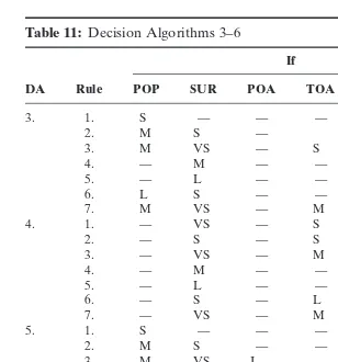
It appears that regions with less than 20,000 inhabitants have a tourist income multiplier that is lower than 0.5. A medium-sized region (between 20,000 and 150,000 people) and with a surface between 500 km2 and 10,000 km2 has a multiplier value of less
than 0.5, whereas a large region (more than 150,000 inhabitants) and with the same surface class has a multiplier value that is higher than 0.9. Finally, a region with a medium-sized number of inhabitants and a small surface (smaller than 500 km2) and a small
Table 10: Reducts of condition attributes and their frequency (adjusted codification)
Attribute Frequency (%)
1. Type of documentation 13 (38.2%)
2. Year of collection of data 6 (17.6%)
3. Research method 4 (11.8%)
9. Population size 519 (41.2%)
4. Surface 616 (35.3%)
5. Geographic feature of the area 313 (17.6%)
6. Political autonomy 715 (35.3%)
7. Number of tourist arrivals 416 (29.4%)
8. Largest country share 619 (36.6%)
10. Type of tourist attractiveness 1014 (41.2%) Reducts of condition attributes:
with meta-variables: {2,7,10}, {2,6,10}, {1,4,10}, {1,6,8,9}, {2,6,8}, {2,4}, {6,8,9,10}, {1,6,9,10}, {1,5,7,10}, {1,5,6,10}, {1,6,7,10}, {1,4,8}, {1,3,4}, {2,3,10}, {1,3,10}, {1,4,9}, {1,4,7}, {1,4,5}, {2,3,8}, {1,3,8}
without meta variables: {5,7,8}, {3,8,10}, {3,7,10}, {3,6,10}, {5,6,8}, {6,7,8}, {3,4,10}, {4,7,8}, {4,5,8}, {3,6,8}, {3,4,8}, {3,4,7}, {3,4,6}, {3,7,8}
Note:For other variables than meta-variables this table first indicates the frequency of their occurrence in reducts with meta variables and second, the frequency of their occurrence in reducts without meta-variables.
(more than 700,000) have a multiplier that is higher than 0.9. Finaly, the same small region with an intermediate tourist inflow has a multiplier value smaller than 0.5, if the share of tourists from one single country is less than 50 percent, while it has a multiplier value larger than 0.9, if this share is higher than 50 percent.
Table 11: Decision Algorithms 3–6
If Then
DA Rule POP SUR POA TOA LCS ATR TIM
3. 1. S — — — — — S
2. M S — S
3. M VS — S — — S
4. — M — — — — M
5. — L — — — — L
6. L S — — — — L
7. M VS — M — — L
4. 1. — VS — S — — S
2. — S — S — — S
3. — VS — M S — S
4. — M — — — — M
5. — L — — — — L
6. — S — L — — L
7. — VS — M M — L
5. 1. S — — — — — S
2. M S — — — — S
3. M VS I — — — S
4. — M — — — — M
5. — L — — — — L
6. L S — — — — L
7. M VS NI — — — L
6. 1. S — — — — — S
2. M S — — — — S
3. M VS — — — NC S
4. — M — — — — M
5. — L — — — — L
6. L S — — — — L
7. M VS — — — SU L
Note:The geographical areas meeting the respective rules are:
3.1, 5.1, 6.1 Alonnisos, Niue, Cook-Islands 3.6, 4.6, 5.6, 6.6 Singapore 3.2, 5.2, 6.2 Tonga 3.7, 4.7, 5.7, 6.7 Bermuda 3.3, 5.3, 6.3 Kiribati 4.1 Niue, Kiribati 3.4, 4.4, 5.4, 6.4 Okanagan, Bahamas, Vanuatu 4.2 Tonga 3.5, 5.5, 4.5, 6.5 Turkey 4.3 Alonnisos
6.D. Evaluation of the Results
The rough-set approach is a decision-theoretic classification tool, which can be properly used in a semiquantitative meta-analytical setting.
of the tourist region concerned. A positive contribution to the tourist multiplier is also offered by the population size, the number of tourists, and the tourist market share of the major country of origin. From a methodological perspective, rough set analysis has the important potential to construct a set of reducts of case study features. Such reducts contain sets of characteristics that discrimi-nate as much as possible between the various case study results. In this way it is possible—through elimination of redundancy—to describe the available information—following logical rules—with a lower number of attributes. A decision algorithm based on a reduct may be regarded as an alternative but simpler information system for mapping out the variety in case study characteristics. Rough-set analysis is particularly useful for categorical informa-tion represented in ranges or distinct classes. In case of ratio information, one may still use rough set approaches, but then it is preferable to present this information in a large number of distinct classes.
Finally, it is clear that an extension of the original set of objects (cases) with a new one leads to additional information that will impact on the composition of the reducts and, hence, on the structure of the decision algorithm. This is plausible, as new infor-mation should lead to adjusted decision rules; otherwise, the new information is redundant. This means that it is necessary to include in a rough-set analysis all available information on all available objects or case studies.
In the next section, we will use the results from the above rough-set analysis to make the best possible and most plausible prediction of the tourism income multiplier for another region, for which documented information does not exist (i.e., there are no meta variables).
7. USING META-ANALYSIS TO ESTIMATE UNKNOWN TOURIST INCOME MULTIPLIERS
In this final section we will use the results from both the regres-sion analysis and the rough-set analysis to assess the unknown tourist income multiplier for another region, viz. the Greek island of Lesvos. The available relevant background information on this island is given in Table 12.
Table 12: Background Information on Lesvos
Attribute
Population (in 1991) 86,907
Surface 1630 km2
“Island” Lesvos is an island
Political autonomy Lesvos belongs to Greece Number of tourists
Upper estimation 347,545
Lower estimation 47,347131,511578,858
Share 56.4% of the tourists are Greek
Type of holiday Both sun and culture holidays Tourist index
Lower estimation 0.91
Upper estimation 4.00
Note:upper estimation of the number of tourists5total number of people that arrived in 1991 by boat or airplane on Lesvos.
Lower estimation of the number of tourists5number of people that arrived in 1991 by charter flight (foreigners) added with the number of Greeks that in 1990 stayed at least 1 night in a hotel on Lesvos.
Share5quotient of the number of Greeks that stayed in 1990 at least 1 night in a hotel and the total number of people that stayed in 1990 at least 1 night in a hotel in Lesvos (3100%).
Lower estimation of tourist index5quotient of the lower estimation of the number of tourists and the number of inhabitants.
Upper estimation of tourist index5quotient of the upper estimation of the number of tourists and the number of inhabitants.
Table 13: Meta-Analytic Prediction of Tourist Income Variables for Lesvos by Means of Regression Analysis
No. Prediction dg Interval No. Prediction dg Interval
1 0.73 (0.33) 8 [20.029; 1.49] 13L 0.75 (0.32) 7 [20.037; 1.50] 2 0.64 (0.25) 7 [20.042; 1.24] 13H 0.84 (0.33) 7 [0.066; 1.62] 3 0.68 (0.30) 7 [20.039; 1.40] 14L 0.65 (0.15) 6 [0.28; 1.02] 4 0.58 (0.16) 6 [0.19; 0.98] 14H 0.79 (0.16) 6 [0.40; 1.17] 5 0.74 (0.39) 9 [20.14; 1.63] 15L 0.62 (0.28) 7 [20.043; 1.29] 6 0.63 (0.29) 8 [20.030; 1.29] 15H 0.76 (0.28) 7 [0.10; 1.41] 7 1.11 (0.26) 7 [0.53; 1.69] 16L 0.55 (0.18) 6 [0.12; 0.98] 8 0.96 (0.23) 6 [0.41; 1.52] 16H 0.67 (0.17) 6 [0.25; 1.10]
Note:standard deviations are given in brackets. no5number of regression equation (see Table 2).
L5the number of tourists arriving on Lesvos is underestimated. H5the number of tourists ariving on Lesvos is overestimated. dg5number of degrees of freedom.
almost certainly tourists. Nationalities, places of origin, and rea-sons of traveling of people belonging to the first group are, how-ever, unknown. Therefore, we choose the number of people be-longing to the first and the second group as an upper bound of the number of tourists coming to Lesvos in a year. The lower bound of the number of tourists is assessed as follows. The number of Greeks staying in a hotel is known. If we suppose that they are all domestic tourists, we may assume that this number aug-mented by the number of people arriving by charter flight is a lower bound of the number of tourists arriving in Lesvos.
Regression models that use the upper estimate of the number of tourists appear to lead to higher predictions of the tourist income multiplier than regression models that use the lower esti-mate of the number of tourists. The differences between the re-spective predicted values are 0.09, 0.14, 0.14, and 0.12 for the models 13 to 16 in Table 4.
so that it is not possible to predict Lesvos’ multiplier value on the basis of one of the decision rules. Second, Lesvos obeys the predecessor of exactly one of the decision rules. This outcome is most desirable, because then the decision rule concerned simply gives us one prediction interval. Third, Lesvos obeys two or more predecessors. If, in that case, the rules concerned prescribe differ-ent values of the multiplier; the decision algorithm is inconsistdiffer-ent with respect to Lesvos. Let us begin considering the decision algorithms that are based on the first classification. Decision algo-rithm 1 predicts a multiplier value between 0.5 and 1.0: Lesvos obeys the value intervals of the attributes contained in the fifth decision rule. The second algorithm is inconclusive with respect to Lesvos, as Lesvos does not obey these predecessors. Decision algorithms 3 up to 6 are based on the second classification (see Table 9). Lesvos obeys a predecessor of a rule that forms a part of algorithms 3, 5, and 6. According to this rule Lesvos has a multiplier value less than 0.5. Finally, algorithm 4 is inconclusive with respect to Lesvos.
As a consequence, regression models that take account of this special position of Turkey are more plausible. Furthermore, the tourist models are to be preferred to base models, as the first ones have a higher information content. As a consequence, our attention will be focused on regression models 14 and 16. The estimates of the coefficients of model 16 are plausible but those of model 14 are not. Therefore, according to model 16, we choose the value of 0.67 as an upper bound of the average tourist income multiplier of Lesvos.
8. RETROSPECT AND PROSPECT
In conclusion, despite the limited number of case studies, meta-analytic techniques are able to assess values of unknown base variables, provided relevant background information on case stud-ies is available. A major advantage appears to be that meta-analysis may mean a significant saving in research efforts. New case studies do not always necessarily require extensive field work to arrive at first plausible assessments of response variables, as tentative valid insights can already be acquired from previous case studies, taking into account the site-specific conditions and the particular methodology used.
In this context, recent developments in areas outside of the conventional domains of statistics may provide new useful ways forward. Nonparametric techniques, and especially various forms of soft modeling, would seem to offer a viable way of handling empirical research, when there is lack of instant information on the case study at hand. A promising solution to problems of comparing differing measuring procedures and those associated with making distributional assumptions, for instance, is the adoption of rough and fuzzy set analysis (see Greco et al., 1995). Developments here may provide interesting scope for further work in more policy-oriented areas which often involve considerations on a multiplicity of performance measures. These developments are important if the applications of meta-analysis are to provide a balanced output for policy assessment.
REFERENCES
Archer, B.H. (1976) The Anatomy of a Multiplier.Regional Studies.10:71–77.
Baaijens, S.R. (1996) Raming van Toeristische Inkomensmultipliers met Meta-Analyse, M.A. Thesis, Free University, Amsterdam.
Button, K.J. (1994) Evaluation of Transport Externalities: What Can We Learn Using Meta-Analysis? Paper presented to the Advanced Studies Institute on Transport, Environment and Traffic Safety, Tinbergen Institute and Department of Spatial Economics, Free University, Amsterdam.
Button, K.J. (1995) The Impacts of Transport: What Can We Learn Using Meta-Analysis. Regional Studies, 29:507–517.
Button, K.J., and Nijkamp, P. (1996) Environmental Policy Assessment and the Usefulness of Meta-Analyses.Socio-Economic Planning Sciences.
Coccossis, H., and Nijkamp, P. (Eds.). (1995)Sustainable Tourism Development.Aldershot: Avebury.
Cook, T.D., and Leviton, L.C. (1980) Reviewing the Literature: A Comparison of Tradi-tional Methods With Meta-analysis.Journal of Personality, 48:449–472.
Cook, Th.D., Cooper, H. Cordray, D.S., Hartmann, H., Hedges, L.V., Light, R.J., Louis, Th.A. and Mosteller, F. (1992).Meta-Analysis for Explanation.New York: Sage. Cooper, H., and Hedges, L.V. (Eds.).The Handbook of Research Synthesis.New York:
Russell Sage Foundation.
Economist, The.(1991) Under the Metascope, 319:93–94.
Fiske, D.W. (1983) The Meta-analytic Revolution in Outcome Research.Journal of Con-sulting Psychology51:65–70.
Fletcher, J. (1989) Input–Output Analysis and Tourism Impact Studies.Annals of Tourism Research, 16:514–529.
Funtowicz, S.O., and Ravetz, J.R. (1990)Uncertainty and Quality in Science for Policy. Dordrecht: Kluwer Academic.
Glass, G.V., McGaw, B., and Smith, M.L. (1981)Meta-Analysis in Social Research, Beverly Hills: Sage.
Greco, S., Matarazzo, B., and Slowinski, R. (1995) Rough Set Approach to Multi-Attribute Choice and Ranking Problems, ICS Research Report 38/95, Warsaw University of Technology, Warsaw.
Hedges, L.V., and Olkin, I. (1985) Statistical Methods for Meta-Analysis, New York: Academic Press.
Hunter, J.E., Schmidt, F.I., and Jackson, G. (1982)Advanced Meta-Analysis: Quantitative Methods for Cumulating Research Findings across Studies.Beverly Hills: Sage. Light, R.J., and Pillemer, D.B. (1984)Summing Up—The Science of Reviewing Research,
Cambridge, MA: Harvard University Press.
Mann, C. (1990) Meta-analysis in the Breech.Science249:476–480.
Matarazzo, B. (1996) Basic Principles of Rough Set Analysis.Meta-Analysis of Environmen-tal Strategies and Policies at a Meso Level(P. Nijkamp, JC.M.J. van den Bergh, and P. Pepping Eds.). Brussels: Report European Commission.
Mitra, A., Jenkins, G.D., and Gupta, N. (1997) A Meta-analytic Review of the Relationship Between Absence and Turnover.Journal of Applied Psychology879–889. Morris, C.T., and Adelman, I. (1988)Comparative Patterns of Economic Development
1850–1914, Baltimore: The John Hopkins University Press.
Nijkamp, P., and Blaas, E. (1994)Impact Assessment and Evaluation in Transportation Planning.Boston: Kluwer.
Pawlak, Z. (1982) Rough Sets,International Journal of Information and Computer Sciences, 11:341–356.
Pearce, D. (1989)Tourism Development.Essex: Longman.
Pearce, D., and Turner, P.K. (1990)Economics of National Resources and the Environment. New York: Harvester Wheatsheaf.
Petitti, D. (1993)Meta-Analysis, Decision Analysis and Cost-Effectiveness Analysis.New York: Oxford University Press.
Pleeter, S. (1980)Economic Impact AnalysisBoston: Kluwer.
Rosenthal, R. (1991)Meta-Analytic Procedures for Social Research.Beverly Hills: Sage. Slowinski, R. (Ed.) (1993)Intelligent Decision Support. Handbook of Applications and
Advances of Rough Sets Theory.Dordrecht: Kluwer.
Smith, V.K., and Kaoru, Y. (1995) Can Markets Value Air Quality, A Meta-analysis of Hedonic Property Value Models.Journal of Political Economy103:209–227. Stanley, T.D., and Jarrell, S.B. (1989) Meta-Regression Analysis.Journal of Economic
Surveys16:161–170.
van den Bergh, J.C.J.M., Matarazzo, B., and Munda, G. (1995) Measurement and Uncer-tainty Issues in Environmental Management: A Survey, TRACE Discussion Paper TI-95-81, Tinbergen Institute, Amsterdam.
Wachter, K.W. (1988) Disturbed by Meta-analysis.Science241:1407–1408.
Walsh, R.G., Johnson, D.M., and McKean, J.R. (1989) Market Values from Two Decades of Research on Recreational Demand.Advances in Applied Economics(A.N. Link and V.K. Smith, Eds.). Greenwich: JAI Press, pp. 106–133.
Wolfe, H. (1986)Meta-Analysis: Quantitative Methods for Research Synthesis.Beverly Hills: Sage.
Case Studies Included in the Meta-Analysis
Archer, B.H. (1977)Tourism in the Bahamas and Bermuda: Two Case-Studies.Cardiff: Bangor Occasional Papers in Economics, no. 10.
Giaoutzi, M., and Nijkamp, P. (1994)Decision Support Models for Regional Sustainable Development.Aldershot: Avebury.
Khan, H., Seng, C.F., and Cheon, WK. (1990) Tourism Multiplier Effects on Singapore. The Annals of Tourism Research, 17:408–418.
Liu, J., Var, T., and Timur, A. (1984) Tourist Income Multipliers for Turkey.Tourism ManagementDecember:280–287.
Milne, S.S. (1987) Differential Multipliers.The Annals of Tourism Research4:499–515. Milne, S. (1992) Tourism and Development in South Pacific Microstate.The Annals
of Tourism Research, 19:1919–212.
Pepping, G., and de Bruijn, M. (1991) Tourism: Emphasis on Selective Development, M.A. Thesis, Free University, Amsterdam.
Var, T., and Quayson, J. (1985) The Multiplier Impact of Tourism in the Okanagan. The Annals of Tourism Research, 12:497–514.
APPENDIX: LIST OF TOPICS FOR THE INVESTIGATION OF THE STUDY REPORTS ON TOURISM
A. Source
B. Geography
number of inhabitants surface
geographical location autonomy
C. Research
economic model used degree of disaggregation year of data collection D. Multiplier values
average income multiplier sectoral multipliers
multipliers for certain groups E. Tourism
number of tourists (arrivals and nights) origin of tourists
seasonality of tourism
accommodation (type, number) expenditure patterns
type of tourist attractiveness F. Economy
expenditure patterns of households expenditure patterns of firms import ratios
sectoral composition of employment and production G. Environment
environmental decay H. Policy