www.elsevier.nlrlocatereconbase
Discussion
Insurance and imperfect financial markets in
Grossman’s demand for health model — a reply
to Tabata and Ohkusa
Bengt Liljas
)Program on Economic EÕaluation of Medical Technology, Department of Health Policy and Management, HarÕard School of Public Health, Boston, USA
( )
LUCHE Lund UniÕersity Centre for Health Economics , Lund, Sweden
Received 7 December 1999; received in revised form 17 January 2000; accepted 25 January 2000
Abstract
In the article by Tabata and Ohkusa, they show that the insurance system set out in w
Liljas Liljas, B., 1998a. The demand for health with uncertainty and insurance. Journal of x
Health Economics 17, 153–170. does not have an optimal solution, and propose a new formulation. It is argued here that even though the new model works mathematically, it has a less realistic economic foundation. Furthermore, generalizing the Grossman model by making the marginal utility of income variable over time is suggested to be more relevant in the case where there are imperfect financial markets, and a simple example is provided. Overall, there seems to be room for further theoretical extensions in the demand for health literature.q2000 Elsevier Science B.V. All rights reserved.
JEL classification: D13; D31; D61; D80; I10; I12
Keywords: Demand for health; Insurance; Imperfect financial markets
)AstraZeneca, S-221 87, Lund, Sweden. Tel.:q46-46-338-017; fax:q46-46-337-169.
Ž .
E-mail address: [email protected] B. Liljas .
0167-6296r00r$ - see front matterq2000 Elsevier Science B.V. All rights reserved.
Ž .
1. Introduction
The demand for health is one of the most central topics in the area of health economics, and the classical model derived by Michael Grossman is one of its
Ž .
cornerstones Grossman, 1972 . However, theoretical extensions of this model, as well as competing economic models, are still relatively few. An obvious extension was to enter Grossman’s deterministic model into a stochastic framework, and then to investigate the effects of insurance. These were two of the topics that I
Ž .
treated in an article a couple of years ago Liljas, 1998a . In this issue of Journal
Ž .
of Health Economics, Tabata and Ohkusa 2000 show the non-existence of an
optimal solution in my model with social insurance, and propose an alternative formulation. Furthermore, they also extend the stochastic version of the Grossman model by letting the marginal utility of income be variable over time. This paper is structured in the following way; Section 2 discusses Tabata and Ohkusa’s alterna-tive model with insurance, Section 3 examines the cases when the marginal utility of income is likely to be variable over time, and give a simplistic example thereof, and, finally, Section 4 holds some conclusions.
2. A model with insurance
Tabata and Ohkusa elegantly show the non-existence of an optimal solution in
Ž .1
the model with social insurance in Liljas 1998a . This is non-debatable. How-ever, it should be noted that in doing so they rely on the assumption that the
Ž
households’ production functions are homogenous of degree one e.g., that the
.
impact of medicines on health investments is constant and positive;EIrEMt)0 ,
Ž . Ž .2
an assumption also made in Grossman 1972 and Liljas 1998a . Is this necessarily so?
It is not unreasonable to assume that I is concave in M, i.e., that over-con-sumption of medicines will actually decrease an individual’s health. If so, for rather healthy individuals, an increased consumption of medicines will actually decrease rather than increase their health, and for this set of individuals the consumption of medicines is likely to be rather low and constant at optimum, and thusEIrEMts0. The reason why the consumption of medicines for these
individ-Ž
uals is constant does not depend on a tight budget constraint as the cost for
.
medicines for these individuals would be rather low , but rather on the fact that
Ž
when their utility is maximized, their medicine-utilization is optimized i.e.,
1
In proving that the solution does not exist, the authors reformulate the problem in optimal control
Ž
theory terms, rather than to keep it in the original calculus of variations terms applied in both
. Ž
Grossman, 1972 and Liljas, 1998a . Although this is correct as they yield identical solutions, see, e.g.,
.
Kamien and Schwartz, 1991 , it should be noted that finding the non-existence with the original method is not as straightforward.
2
.
EIrEMts0 . Thus, for these individuals, the only way they can increase their
Ž .
health is by increasing their time input TH , and the only time whenEIrEMt/0
Ž .
is when there are uncertain ‘blips’ e.g., sudden exposure to viruses and germs in their health. For old people, where the costs of medication potentially are a large
Ž
part of their budgets,EIrEM will likely be positive as they might consume lesst
.
medications than they would want and need to . Thus, developing the Grossman model by applying household production functions that are not homogenous of degree one and to investigate how this might affect the existence of various insurance systems, could be of interest.3
The alternative type of insurance system suggested by Tabata and Ohkusa
Ž
unfortunately does not correspond to real life very well which they also
acknowl-.
edge , as it suggests that the insurance company should insure the individuals
Ž .
against any time-loss, rather than only working-time-loss, as in Liljas 1998a . The two setups are very similar, with the important difference that the insurance
Ž . Ž .
system proposed by Liljas 1998a is perhaps more realistic, but the one
Ž
suggested by Tabata and Ohkusa holds mathematically true it could also be noted
.
that the Euler equations, not surprisingly, are almost identical .
3. A model with imperfect financial markets
In Grossman’s original model, everything is deterministically determined; the individual knows with certainty the effects of health investments, how long he or she will live, as well as how large his or her life-time income is. As the interest
Ž .
rate is equal for borrowing and saving without any transaction cost , he or she can thusAeven outBthe income over the different periods of life. Obviously, when his or her income is low, he or she will borrow money, and when it is high, he or she
Ž .
will save money. In this case, the marginal utility of income l will be constant. In the case of uncertainty, the individual will no longer know his or her time of death or life-time income. To avoid being in debt at the time of death, the individual might have to save more money in earlier time-periods than in the deterministic case, and as the disposable income then will vary over time, l will be variable — as proposed by Tabata and Ohkusa. However, if the uncertainty is not too high, and the individuals’ expectations are not too far off, l will still remain fairly constant.
A more likely instance when l will vary over time, is when the financial
Ž
markets are imperfect. That is, what if the individual contrary to Grossman’s
.
original model no longer can borrow and save money at the same and constant
3 Ž .
The assumption of constant returns to scale was also discussed in Erlich and Chuma 1990 , who
Ž .
argue that this introduces a type of indeterminacy a ‘bang-bang’ control problem for the optimal investment in health. However, introducing diminishing returns to scale for investments in health as
Ž .
Ž . Ž .
interest rate and when there are transaction costs involved ? As an overly simplistic baseline case, assume that the individual can neither borrow nor save money.4 The individual will then have a binding budget constraint for each time-period, and as there are no financial markets at all, there are no possibilities of earning interest so the interest rate falls out of the optimization problem.
In this case, the individual’s utility maximization problem under uncertainty and with imperfect financial markets can be written:
T Hmax
yut
Max
H H
uŽ
ftH , Z et t.
g H d H d t ,Ž
t.
tŽ .
10 Hmin
Hmax
s.t. Rts
H
Ž
pt tIqq zt tqw TLt t. Ž
g H d H ;t.
t ;t ,Ž .
2Hmin
˙
HtsItydt
Ž
H ,Qt t.
H .tŽ .
3From Eqs. 1 and 2, the Lagrange function can be formulated as:
T
yut
Ls
H
E uŽ
ftH , Zt tŽ
X ,Tt t.
.
e yl ptŽ
t tI M ,THŽ
t t.
qq Zt tŽ
X ,Tt t.
0
qwt
Ž
VyftHt.
.
d t.Ž .
4Hence, by using Eq. 4 as the objective function, the Hamiltonian reads:
yut
JsE u
Ž
ftH , Zt tŽ
X ,Tt t.
.
e yl ptŽ
t tI M ,THŽ
t t.
qq Zt tŽ
X ,Tt t.
qwt
Ž
VyftHt.
.
qmtŽ
I M ,THtŽ
t t.
ydtŽ
H ,Qt t.
Ht.
Ž .
5 The first-order conditions of this optimization problem are:EJ Eu EZt yut EZt
sE e yltqt s0,
Ž .
6EXt EZt EXt EXt
EJ Eu EZt yut EZt
sE e yltqt s0,
Ž .
7ETt EZt ETt ETt
EJ EIt EIt
s yl pt t qmt s0,
Ž .
8EMt EMt EMt
EJ EIt EIt
s yl pt t qmt s0,
Ž .
9ETHt ETHt ETHt
EJ Eu Edt
yut
ym
˙
ts sftž
E e qltwt/
ymtE dtq H .tŽ .
10EHt Eht EHt
4
Ž .
For an elaboration of the deterministic case when the individual can also save money, see Liljas
Ž .
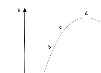
Fig. 1. Graphical illustration of a concave function of income over time Rt and the average life-time
Ž .
income R .
From Eq. 8, assuming homogeneity of degree one, we get: mtsl pt t, and
˙
Ž . Ž . Ž .
differentiating this with respect to t yields m
˙
trmt s ltrlt q p˙
trpt . Finally, substituting these equations into Eq. 10 and rearranging gives us:Eu Edt
yut
˙
ft
ž
wtqE e rlt/
sE dtq Ht ptyp˙
typ lt trlt.Ž .
11Eht EHt
5 Ž .
Thus, compared to the solution in Tabata and Ohkusa their Eq. 17 , there are
Ž . Žryu.t yut
four changes in Eq. 11. 1 The discount factor has changed from e to e .
Ž .2 The marginal utility of income has changed from l to lt. 3 The discountŽ .
˙
Ž .
rate, r, has disappeared. 4 An additional term,yp lt trlt, has appeared, where
˙
lt is the time-change of how binding the budget constraint is. Since r is positive,
Ž .
the first and third change decreases the marginal benefit MB and the marginal
Ž .
cost MC , respectively. The sign of the second change depends on the level of
Ž .
income, R , which in turn determinest lt and affects MB . For the fourth change,
˙
˙
Ž . Ž .
it is valid that: signyp lt trlt ssignylt , and affects MC, since bothpt and
lt are positive.
To be able to conclude how imperfect financial markets affect the demand for
˙
health at optimum, we need to know the size of lt and the sign of lt. In Grossman’s original model, the individual could even out the life-cycle income at
Ž
the level R. Using the well-known life-cycle hypothesis Ando and Modigliani,
. Ž .
1963 , where R is concave over time indicating thatt lt is convex , R will att
Ž
certain time-periods lie above R, twice equal R, and otherwise lie below R see
Eu Edt
5This equation reads:f wqE eryutrl s rqE dq H pyp˙.
t
ž
t/ ž
t t/
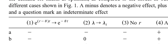
t tTable 1
Ž .
A summary of the four changes 1 and 2 affecting MB, and 3 and 4 affecting MC and their effect on the demand for health at optimum, as compared to the model in Tabata and Ohkusa, for the seven different cases shown in Fig. 1. A minus denotes a negative effect, plus a positive effect, zero no effect, and a question mark an indeterminate effect
Žryu.t yut ˙
Ž .1 e ™e Ž .2 l™lt Ž .3 No r Ž .4 Add:yp lt trlt H
a y y y q y
b y 0 y q y
c y q y q 0
d y q y 0 q
e y q y y q
f y 0 y y ?
g y y y y ?
.6 Ž .
Fig. 1 . Here, there are seven different cases a to g where changes two and four, above, affect the demand for health at optimum.
Comparing Eq. 11 to Eq. 17 in Tabata and Ohkusa is difficult since we have two changes affecting both MB and MC. Some of the conclusions therefore rest on the strong assumption that two changes in opposite direction within either MB or
7 Ž .
MC cancel out. Given this assumption, the following holds see Table 1 : for
Ž . Ž . Ž .
cases a and b , the demand for health at optimum is here lower, for cases d
Ž .
and e , it is higher, and for all other cases, it is zero or indeterminate. This suggests that when income is low but increasing, the demand for health at optimum is smaller. In these cases, the individual will postpone his or her investments in health as long as he or she believes that his or her income will
Ž
increase over time since the opportunity cost of investments in health then will
.
decrease over time . Similarly, when income is high but decreasing, the demand for health at optimum is higher. According to the life-cycle hypothesis, the individual would here invest more in his or her health during the later parts of life.
4. Discussion
In this paper, I have tried to scrutinize the insurance system and the introduc-tion of a variable marginal utility of income, both applied to Grossman’s demand for health model, proposed by Tabata and Ohkusa.
6
This shape of the dynamics of income is naturally an assumption, but shows many of the likely patterns.
7
Ž .
Tabata and Ohkusa are correct that an optimal solution to the insurance system
Ž .
suggested by Liljas 1998a does not exist. However, the alternative insurance
Ž .
system suggested although correctly specified mathematically is not as appeal-ing, as it rests on the rather unrealistic assumption that all time loss is insured — even when the individual is not working. As the non-existence of the insurance
Ž .
system suggested by Liljas 1998a is based on that the households’ production functions are homogenous of degree one, a possible new extension would be to relax that assumption. It is also argued here that the underlying reason for a variable marginal utility of income is of great importance. Uncertainty may indeed affect the individuals’ opportunities to equate his or her income over the life-cycle. However, imperfect financial markets will likely have greater implications on the individuals’ budget constraints. A simplistic example where the individual could neither borrow nor save money was presented, and the demand for health was shown to largely depend on the level of income, and the change of income over time. An interesting development in this area would be to allow for both savings and borrowing, but at different interest rates.
The introduction of insurance and a time-dependent marginal utility of income are both important contributions to Grossman’s demand for health model. Both this and the article by Tabata and Ohkusa have given new insights on these topics. However, it seems obvious that there is room for further theoretical developments and extensions to the area of demand for health.
References
Ando, A., Modigliani, F., 1963. The life cycle hypothesis of saving: aggregate implications and tests. American Economic Review 53, 55–84.
Erlich, I., Chuma, H., 1990. A model of the demand for longevity and the value of life extension. Journal of Political Economy 98, 761–782.
Grossman, M., 1972. On the concept of health capital and the demand for health. Journal of Political Economy 80, 223–255.
Grossman, M., 1999. The human capital model and the demand for health. NBER Working Paper 7078.
Kamien, M., Schwartz, N., 1991. Dynamic Optimization: The Calculus of Variations and Optimal Control Theory in Economics and Management. Elsevier, New York.
Liljas, B., 1998a. The demand for health with uncertainty and insurance. Journal of Health Economics 17, 153–170.
Liljas, B., 1998b. The demand for health, life-time income, and imperfect financial markets. Studies in Health Economics 25, Department of Community Medicine and the Institute of Economic Re-search, Lund University, Sweden.
Tabata, K., Ohkusa, Y., 2000. Correction note on The demand for health with uncertainty and
Ž .