A MATHEMATICAL MODEL OF DENGUE
INTERNAL TRANSMISSION PROCESS
N. Nuraini, E. Soewono, K.A. Sidarto
Abstract.In this paper we formulate a mathematical model of internal process of dengue virus transmission in the human body. We analyze the dynamic of dengue virus using a system of differential equation. We obtain a local stability of equilibrium for this model base on a threshold parameter. In particular, we prove the stability result for a free-virus and abundance of virus-states. Finally, numerical simulation of the model are performed to study the behaviour of the system for a short period of time.
1. INTRODUCTION
Dengue viral infections are one of the most important mosquito borne diseases in the world. They may give rise dengue fever (DF), dengue haemorrhagic fever (DHF), or dengue shock syndrome (DSS). The incidence of DHF has increased dramatically in recent years with approximately five times more cases reported since 1980 than previous 30 years. Dengue may be caused by one of the dengue viral serotypes, DEN-1, DEN-2, DEN-3 and DEN-4. Although serological surveys conducted in Indonesia showed that DEN-1 and DEN-2 were prevalent serotypes until the late 1980s, the DEN-3 serotype has been the predominant serotype in the recent outbreaks [4] and [6]. In fact, DEN-3 has been associated with severe dengue epidemics and it has been suggested that the DEN-3 virus may have certain char-acteristic that make it more virulent. Generally, infection with one serotype confers future protective immunity against that particular serotype but not against other serotypes. Furthermore, when infected for a second time with different serotype, a more severe will occur [3]. After the bite of an infected mosquito, the dengue virus enters the body and replicates within cell of the mononuclear phagocyte lineage
Received 1 May 2006, revised 12 December 2006, accepted 20 December 2006. 2000 Mathematics Subject Classification: 92D30
Key words and Phrases: mathematical model, equilibrium points, threshold parameter, numerical sim-ulation
(macrophages, monocytes, and B cell). The incubation period of dengue infections is 7-10 days. A viraemic phase follows where the patient becomes febrile and infec-tive. Thereafter, the patient may either recover or progress to the leakage phase, leading to DHF and/or dengue shock syndrome [6]. To estimate the duration of viremia, researchers assumed detectable viremia started on the day prior to onset of illness and ended on the last day in which it was detected. For example, if a child was admitted on the third day of illness and virus was detected until the fifth day of illness (study days 1-3), then the viremia duration was 5 days. Duration of Dengue viremia ranged from 1 to 7 days [8]. This fact is address the question does the mathematical model can show this phenomenon? In this paper we want to formulate the mathematical model of dengue internal process transmission based on some assumptions. This formula describes in section 2. In the section 3 we analyze the model with dynamical analysis near the equilibrium point based on a threshold number. The numerical result explained in the section 4. And the last section we discuss about the result of this work and explain the viremia phenomena from the numerical simulation.
2. FORMULATION OF THE MODEL
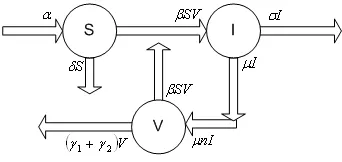
In order to derive the equations of the mathematical model, we assumed that dengue viruses are virulent, and no other microorganism that attack the body. It is believed that mainly support dengue virus infections (in vivo) are monocytes, macrophages and other cells of reticuloendothelial origin [5]. We define this cell as susceptible cell denoted by S(t). The infected cell compartment is I(t), and the free virus particles isV(t). This diagram below describe the transmission virus in the human body based on this model.
Figure 1: Transmission Diagram
The dynamic of the cell population given by equation (1- 4).
dS(t)
dt = α−βS(t)V(t)−δS(t), dI(t)
dV(t)
dt = µnI(t)−γ1V(t)−γ2V(t)−βS(t)V(t)
Equations (1) represent the rate of susceptible, infected cells and also a virus. In this model we used a simplest assumption that susceptible cell as uninfected cells are produced at a constant rate, α, and die at a rate δS(t). Free virus particles infect susceptible cells at rate proportional to the product of their abundances,
βS(t)V(t). The constant rate, β, describes the efficacy of this process, including the rate at which virus particles find susceptible cells, the rate of virus entry, and the rate and probability of successful infection. Infected cells produce free virus at a rate proportional to their abundance, µnI(t), with n is the multiplication rate and free virus particles are removed from the system at rate (γ1+γ2)V(t), whereγ1 is natural death rate of virus andγ2 is the death rate of virus by T-cells. The free virus also move to the susceptible cells compartment as βS(t)V(t). The infected cells die at a rateσI(t). We consider this model as a model of virus dynamic that described in [7]. In the next section the condition for the existence of equilibria of the equations (1) are established.
3. ANALYSIS OF THE MODEL
First, we note that the feasible region of biological interest
Ω ={(S, I, V) :S, I, V ≥0}
is positively invariant of system (1), since the vector field on the boundary of Ω does not point the exterior of Ω. We can immediately identify two equilibrium points of system (1), which belong to the boundary of Ω; E1 = (αδ,0,0), and
than one other infected cell. If on the other hand, R0 > 1, then every infected cell will on average produce more than one newly infected cell [7]. In this model, before infection, we have I = 0, and V = 0, and susceptible cells are at equilibrium
S = α
δ. Denote by t = 0 the time when infection occurs. Suppose that infection
occurs with a certain amount of virus particles,V0. Thus the initial condition are
S0 = αδ, I0 = 0, and V0. The rate at which one infected cell gives rise to new
This number provides a key threshold quantity which will be used for stability analysis of the equations (1) throughout the paper.
The stability properties of VFE is given in the next theorem.
Theorem 3.1. The virus-free equilibrium E1 is locally asymptotically stable if
R0<1 and unstable otherwise.
Proof. To determine the local stability ofE1, the Jacobian of equations (1) is eval-uated at the VFE to yield
DE1 =
The eigenvalues ofJE1 are−δ and roots of polynomial
p(s) =s2+ (σ+γ1+γ2+ locally asymptotically stable (see appendix A.1). This complete the proof of the theorem.
and
(R0−1)>0 what can be recast asR0>1.
Linearizing system (1) near the equilibriumE2 we have
DE2 = Using Routh-Hurwitz criterion (see Appendix A.2) the all roots of polynomial
q(s) have negative real parts if and only ifab > cor
We can summarize these findings in the following theorem.
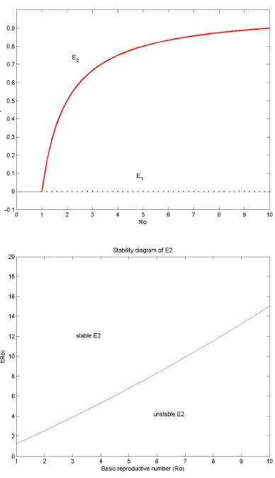
Theorem 3.2. The equilibrium E2exist ifR0>1, and it is locally asymptotically stable if and only if satisfy the condition (4).
In Figure (2) we show the bifurcation diagram for the equilibria of model (1) with respect to R0. For R0 > 1 we plot the proportion of infected cells I∗ given in Eq.(3), and we illustrate the condition (4) under the fixed parameters
4. NUMERICAL SIMULATION
Now, we discuss the numerical simulation of the model as the parameters in the system are varied. We have a generate numerous range of parameter’s value and generally we have the result as in Figure 3. In Figure 3 the maximum number of infected cells is 254.2898 and achieved at the time 4.4254 days. The maximum num-ber of virus load is 1.8.103at the same time as the infected cells. Analyzing Figure 3, the basic model of virus dynamics shows an exponential growth phase of free virus and infected cells followed by a peak and decay to an equilibrium. Uninfected cells stay initially constant, then decline sharply to a nadir and subsequent recover to their equilibrium value. Virus growth will not continue indefinitely, because the supply of uninfected cells is limited. There will be a peak of virus load and decay to its equilibrium.
5. DISCUSSION
In this paper, we have derived and analysis the dengue internal transmission process model. We have found that the local stability of virus-free equilibrium has been proved for R0 < 1. A threshold condition is R0 = 1, and for R0 < 1 the virus-free equilibrium is locally asymptotically stable and unstable otherwise.
There is one equilibrium of abundance of susceptible cells, infected cells and free virus,E2. The condition for this equilibrium to exist has proved to beR0>1. The stability result of E2 is formulated in theorem 3.2, where it is summarized in (4) conditions.
We have also studied the system (1) numerically, and results for different values of parameters are illustrated in figure 3. As it was noted in section 1, this model in this paper simulate the phenomena that the dengue virus may disappear from human blood body system at least in 14 days after the bite of mosquito.
Appendix A.1. Stability.
Consider a general autonomous vector field
˙
x=f(x), x∈ Rn. (5)
An equilibrium points of (5) is a point ¯x∈ Rn such that
f(¯x) = 0.
Suppose all of eigenvalues ofDf(¯x) have negative real parts. Then the equilibrium points x= ¯xof the nonlinear vector field (5) is asymptotically stable ( see detail and proof in [9] ).
Appendix A.2. Routh-Hurwitz Criteria.
Suppose that A is a stability matrix. Once the characteristic polynomial of A has been calculated, there are a variety of criteria which can be applied to determine whether or not all the roots have negative real parts. Perhaps the most useful of these are criteria of Hurwitz. Consider the equation
|λI−A|=λN +a1λN−1+...+aN−1λ+aN = 0 (6)
whereak is taken to be zero fork > N. A necessary and sufficient condition
h1=|a1|, h2=
formed from the preceding array, be positive. Using the foregoing criteria, a neces-sary and sufficient condition thatλ3+a1λ2+a2λ+a3be a stability polynomial is thata1, a2, a3>0 anda1a2> a3.By this we mean that the roots of the polynomial have negative real parts [1].
Acknowledgement. The authors would like to thank Yudi Adi and Hengki Tas-man for fruitful discussion during this research. This research is funded by Math-ematical Scientific Activities 2005 Department Mathematics ITB.
REFERENCES
1. R. Bellman,Introduction to matrix analysis, Mc Graw Hill, New York, 1970. 2. O. Diekmann and J.A.P. Heesterbeek, Mathematical epidemiology of infectious
diseases,John Wiley and Son. New York, 2000.
3. M.G. Guzman and G. Kouri, “Dengue: an update”,The Lancent Infectious Diseases
2(2002).
4. S.B. Halstead, F.X. Heinz, A.D.T. Barrett, and J.T. Roehrig, “Dengue virus: molecular basis of cell entry and pathogenesis”,Vaccine23(2005), 849 - 856. 5. I. Kurane and T. Takasaki,“Dengue fever and dengue haemorrhagic fever:
chal-lenges of controlling an enemy still at large”,Rev. Med. Virol11(2001), 301-311. 6. G.N. Malavige, S. Fernando, and D.J. Fernando, , Seneviratne, S.L.,“Dengue
viral infections”,Postgrad. Med. Journal80(2004), 588 - 601.
7. M.A. Nowak and R.M. May,Virus dynamics; mathematical principles of immunology and virology,Oxford University Press Inc., NY 2000.
8. D.W. Vaughn, S. Green, S. Kalayanarooj, B.L. Innis, S. Nimmannitya, S. Suntayakorn, T.P. Endy, B. Raengsakulrach, A.L.Rothman, F.A. Ennis, and A. Nisalak, “Dengue viremia titer, antibody response pattern, and virus serotype correlate with disease severity”,The Journal of Infectious Diseases181(2000), 2 - 9 . 9. S. Wiggins,Introduction to applied nonlinear dynamical systems and chaos,Springer
- Verlag. New York Inc, 1990.
N. Nuraini: Industrial and Financial Mathematics Research Group, Faculty of Mathe-matics and Natural Sciences, Institut Teknologi Bandung, Bandung 40132, Indonesia. E-mail: [email protected].