00074918.2015.1016569

(1)

Full Terms & Conditions of access and use can be found at

http://www.tandfonline.com/action/journalInformation?journalCode=cbie20

Bulletin of Indonesian Economic Studies

ISSN: 0007-4918 (Print) 1472-7234 (Online) Journal homepage: http://www.tandfonline.com/loi/cbie20

Gender Discrimination in Earnings in Indonesia: A

Fuller Picture

Kitae Sohn

To cite this article: Kitae Sohn (2015) Gender Discrimination in Earnings in Indonesia: A Fuller Picture, Bulletin of Indonesian Economic Studies, 51:1, 95-121, DOI:

10.1080/00074918.2015.1016569

To link to this article: http://dx.doi.org/10.1080/00074918.2015.1016569

Published online: 30 Mar 2015.

Submit your article to this journal

Article views: 162

View related articles

(2)

* I am grateful to the two anonymous referees for their helpful comments and suggestions.

GENDER DISCRIMINATION IN EARNINGS IN INDONESIA:

A FULLER PICTURE

Kitae Sohn* Konkuk University, Seoul

This article analyses data from the 2007 Indonesia Family Life Survey in order to decompose the gender gap in earnings into explained and unexplained gaps, not only at the mean but also across the entire distribution. Women earned about 30% less than men, in both paid work and self-employment. The explained gap accounts for only about a quarter of the gap in paid work but for about half of the gap in self-employment. When the decomposition is made across the earnings distribu-tion, the total gap decreases with earnings in both paid work and self-employment, and both conditional and unconditional on characteristics. In both employment sec-tors, the explained gap remains similar across the distribution, and therefore the un explained gap drives the decrease in the total gap. The unconditional decom-position across the distribution provides great insight into the dynamics that are obscured in results derived from decomposition at the mean.

Keywords: gender, discrimination, earnings, decomposition JEL classiication: J71, J78, O15, O53

INTRODUCTION

Pay discrimination against women has been discussed extensively, particularly since Becker (1957) incorporated discrimination into economic analysis. With the proliferation of microdata on earnings and with Oaxaca’s (1973) and Blinder’s (1973) development of econometric techniques to estimate pay discrimination,

much effort has been made to estimate the existence and magnitude of

discrimi-nation (see Weichselbaumer and Winter-Ebmer 2005, for a review). The conven

-tional technique, Oaxaca–Blinder decomposition (or Oaxaca decomposition, for brevity), decomposes the gender earnings gap into explained and unexplained

parts at the mean. The unexplained part is usually considered to represent dis-crimination, although this is debatable.

Despite the great amount of research on the topic, few attempts have been made to apply this idea to Indonesia. Byron and Takahashi (1989) investigated gender differences in the returns to schooling, but their sample was limited to paid employees in urban Java. Deolalikar (1993) improved on this by analysing nation

(3)

96 Kitae Sohn

Benjamin (1996) did decompose the gender gap among paid employees by survey year (1980 and 1990) and residence area (urban and rural), and found that the unexplained part ranged from 62% to 81%. Subsequently, Utomo (2008, chapter 3) conducted a study on this subject for Indonesia. However, the sample was rather restricted (urban paid employees with tertiary qualiications), and the main ind

-ing was that 36% of the gender gap was unexplained.

Currently, more sophisticated techniques are available—techniques that

decompose the gender gap in earnings across the entire distribution, not just at the mean. Decomposition across the distribution is of great importance because it

elu-cidates which groups experience a large gap and a correspondingly large degree

of discrimination. Such decomposition helps policymakers identify target groups.

For example, when discrimination is driven by low earners, a policy for eliminat

-ing discrimination can target low earners instead of all earners—decomposition at the mean is too crude to allow such targeting. Moreover, decomposition across

the distribution can be made both conditional and unconditional on observable

characteristics (‘characteristics’, for brevity). The unconditional decomposition

does not merely replicate the conditional decomposition in the absence of char-acteristics; the unconditional decomposition can be estimated even in the pres-ence of characteristics. From a policy perspective, the choice of conditioning

characteristics is sometimes important. Every day, however, we observe earnings

unconditional on characteristics; high earners are simply high earners, not high

earners conditional on, say, education. Further, it is dificult to inely identify tar -get groups as the number of characteristics increases: for example, high earners

among married high-school graduates with two children in urban areas. In such

cases, unconditional decomposition better corresponds to casual observation and facilitates policy implementation.

Applying these econometric strategies to decomposing outcomes by gender or

race is not unique to this article. I have used similar strategies in the past (Sohn 2012a, 2012b), but that research was concerned with racial and gender gaps in

academic outcomes. (Sohn 2014 considers the gender gap in earnings, but the data

are from Iowa, in the United States, in 1915.) I have also used information on earn

-ings from the Indonesia Family Life Survey (IFLS), but without considering the gender earnings gap in Indonesia (Sohn 2013, 2015). To the best of my knowledge, this article is the irst to apply econometric strategies to an understanding of the

gender earnings gap for both paid employees and the self-employed in Indonesia. Little light has been shed on the self-employed in the literature. This is particu-larly unfortunate for Indonesia, because the self-employed account for a consider-able proportion of its labour force. According to statistics from the International

Labour Organization, the self-employed (‘own-account workers’ in the data) in Indonesia in 2008 accounted for 57.2% of the sum of paid employees, employers,

and the self-employed.1

(4)

Indonesia is an interesting case because by the study year, 2007, its economy

had experienced sustained economic growth since the late 1960s (save during the 1997–98 Asian inancial crisis). GDP per capita in 2000 rupiah increased by 3.53 times from 1967 to 2007 (Van der Eng 2010). International trade and foreign direct

investment increased substantially, too, infusing more competition into the

econ-omy. Becker (1957) argued that competition reduces discrimination in the labour market. However, Rosén (2003) challenged this argument; with search frictions in the labour market, wage bargaining, and a irm-speciic disutility associated with hiring women, discriminatory irms are more proitable than non-discriminatory irms, driving non-discriminatory irms out of the market. As a result, competi -tion leads to a greater gender earnings gap in the labour market.

This article has four notable features. First, it decomposes the gender gap in earnings not only at the mean but also across the entire distribution. Second, it

considers the self-employed, along with paid employees. Third, it captures the

features of the Indonesian labour market during recent years. Fourth, it involves

an ad-hoc comparison between Becker’s and Rosén’s theories for the Indonesian case, even though these theories are restricted to paid work. The results suggest that the degree of discrimination in paid work and self-employment is similar, and that lower-earning women in both sectors experience greater earnings gaps

and gaps probably stemming from discrimination. Overall, it appears that Rosén’s

theory better its the Indonesian setting.

THE INDONESIAN CONTEXT

It is instructive to understand the socio-cultural context of gender, work, and employment in Indonesia (ADB 2006; Utomo 2008; Van Klaveren et al. 2010). Although the country has witnessed rapid modernisation and signiicant pro

-gress by women in education and the labour market, an amalgam of cultural, reli

-gious, and social norms still restricts women to the domestic sphere. In the past, women’s high status was associated with their privilege of staying home. In addi -tion, Islam continues to promote men as the dominant, protective, and

responsi-ble party in marriage, while women are assigned reproductive and supportive roles. Further, Law 1/1974 on Marriage, which institutionalises gender-role spe

-cialisation, appears to support equal rights in marriage. However, in detail, it des -ignates the husband as the household head and the provider of the family. This

environment maintains the gendered labour-market expectation that women are secondary earners. Moreover, girls raised in this environment are likely to self-fulil this expectation—even before deciding whether to join the labour market— by receiving less education or majoring in feminised (less remunerative) ields. Upon inishing formal education, girls might choose a career path that does not interfere with their domestic roles. Thus, they might work fewer hours and obtain

less labour-market experience and on-the-job training. All these outcomes

poten-tially undermine their earnings. The prospective for women’s earnings becomes

bleaker if employers base their personnel decisions on this stereotype.

This intimate connection between the domestic sphere and the labour market is detailed in Setyonaluri’s (2014) thesis on the determinants of Indonesian wom

-en’s employment exit and return. Statistics from the fourth round of IFLS (IFLS4)

(5)

98 Kitae Sohn

in Indonesia, but most workers would prefer to work in the formal sector. Thus, the informal sector, which requires relatively little human and material capital and permits considerable lexibility in timing, usually receives workers who are

pushed out of the formal sector. Women are more vulnerable than men to changes in economic conditions and are therefore more likely to engage in and move into

the informal sector. When they work in the informal sector, many women work without pay. Even in the formal sector, they work in low-paying, low-skilled

occupations, and they are less represented among higher positions and salary

levels. Furthermore, Indonesian women face a higher risk of unemployment than

Indonesian men and participate less in the labour force. Some statistics derived

from IFLS4 (explained below) are provided in the appendix. Although it is dif

-icult to determine the degree to which the adverse conditions for Indonesian women in the labour market are due to gender discrimination, the results here can

shed some light on this issue.

DATA

The main dataset in this study is IFLS4, from 2007. The irst round of IFLS (IFLS1) took place in 1993 and followed more than 22,000 individuals from 7,224 house

-holds in 13 of the 26 Indonesian provinces at the time. Owing to cost constraints, this sample represented 83% of the Indonesian population in that year. Thereaf

-ter, four follow-up surveys were conducted, in 1997 (IFLS2), 1998 (IFLS 2+), 2000 (IFLS3), and 2007 (IFLS4), and the project is ongoing. I use IFLS4 here because it is the most recent round of the survey and because the economic growth rate in 2007 was one of the highest after the 1997–98 Asian inancial crisis. When an economy experiences high growth, workers who would usually not be able to participate in the labour force in a recession can work for pay. Thus, it is expected that IFLS4 observed more workers with earnings than earlier rounds did and that the vari

-ation of earnings in the year was greater in IFLS4 than in earlier rounds. These features are useful in analysing the gender gap in the lower parts of the earnings

distribution.

IFLS4 is restricted to men and women aged 18–65 whose main activities in the past week were working, trying to work, or helping to earn income (one category in IFLS4). Since agricultural work has distinctive characteristics, workers in agri

-culture, forestry, ishing, and hunting (one category in IFLS4) are excluded. For similar reasons, casual workers in agriculture and non-agriculture are excluded. By design, unpaid workers are excluded. Overall, these exclusions make my

results comparable to those in the literature. Workers are broadly divided into

two groups: paid employees and the self-employed. Paid employees consist of workers in the public and private sectors; employed workers consist of self-employed workers who work alone, those who work with unpaid family mem

-bers or temporary workers, and those who work with permanent workers.

The most important variables are gender and earnings. Earnings refer to hourly

(6)

wages and proits are incredibly large. Therefore, values greater than the 99th percentile in the raw data (Rp 5 million for paid employees and Rp 9 million for the self-employed) are replaced with 1.33 times the 99th percentile. Among the self-employed, 82 men (4%) and 30 women (2%) reported zero or negative proits. Following a previous study (Sohn 2013), I change these values to one to make

their log value zero.

Whenever employment of women is considered, the issue of career interrup

-tions arises. In this article, potential work experience is constructed traditionally: age, minus years of schooling, minus six years. This construction is dificult to apply to women’s employment because it is likely that childbearing and child-rearing will interrupt women’s work experiences. There is no easy way to circum

-vent this issue, and one therefore needs to be aware of upward bias in the variable for women. In IFLS4, each respondent provided his or her tenure; tenure and its squared term are included in my estimations in an attempt to alleviate the effects

of career interruption.

Women’s selection into employment is also of concern. Ideally, this concern

could be addressed by using the inverse Mills ratio; but it is dificult to ind

variables that satisfy the exclusion restrictions, so no attempt is made to counter selection bias. This article’s main contribution to the literature is its comparison

between the results at the mean and across the distribution. At this point, it is unclear how to incorporate sample selection into the decomposition techniques

across the distribution. Hence, it is more consistent to compare both types of

decomposition results without accounting for selection bias. Selection does not

stop at the choice of employment versus non-employment, and it arises based

on the choice of paid work versus self-employment. This article offers a starting point for analysing these issues, in the hope that future research will address fur -ther complications.

The sample size is 3,715 for male paid employees, 2,111 for female paid

employ-ees, 2,034 for male self-employed workers, and 1,518 for female self-employed workers. Unless otherwise stated, sampling weights are applied to make the sam -ple representative, and standard errors are clustered at the sub-district (kecamatan) level to account for arbitrary intra-correlation.

METHODS

Understanding Gender Discrimination

The gender gap in earnings may occur for several reasons, and gender

discrimina-tion is often provided as an explanadiscrimina-tion. Gender discriminadiscrimina-tion can be deined in many ways, but a broad deinition would be treating a woman differently from a man because she is a woman (Posner 1989). On causes of discrimination, at one extreme of invidiousness lies misogyny—such as when a man has a distaste for associating with women in economic exchanges, not founded on any notions of productivity or eficiency. At the other extreme lies inherent uncertainty—the cost of acquiring information on a worker is ininitely costly, so inherent uncertainty

creates economic exchanges based not on individual but on group information. Statistical discrimination is a mild version of this cause.

Another reason for the gender gap in earnings is women’s lower levels of

(7)

100 Kitae Sohn

justiied. However, if the low levels result from discrimination within or outside the labour market, then it is not easy to justify the gap. Bergmann’s (1971) crowd

-ing theory is inluential in this regard. Accord-ing to Bergmann, when women are forced to enter some occupations (to work as a secretary, for example) owing to dis

-crimination, marginal productivity in these occupations is lowered by the enforced abundance of labour supply. If girls anticipate this, they will accumulate lower levels of or different (probably less remunerative) types of human capital than they would otherwise. In this case, discrimination takes place within the labour market; however, discrimination outside the labour market can produce the same results, including the expectation that women quit work upon marriage (the ‘marriage bar’; Goldin 1990, chapter 6) or that women primarily perform housework, regard

-less of their employment status (the ‘second shift’; Hochschild and Machung 1989). Akerlof and Kranton (2010, chapter 3) explain the same phenomenon but use a different mechanism, introducing the concept of identity. At the deeper level, how

-ever, norms associated with men’s and women’s jobs could result from discrimina -tion. The Indonesian socio-cultural context exhibits these aspects.

Discrimination agents include employers, co-workers, customers, government agencies, and others with whom the discriminator has a commercial or regulatory

relationship. For paid employees, any of these groups can discriminate against

women. For the self-employed, by deinition, there is no employer and probably no co-worker to discriminate against women. However, self-employed women

may still face discrimination from the other groups. For example, some custom-ers may not like certain goods and services (construction materials, for

exam-ple) being sold by women. In this case, before entering the labour market, girls may accumulate human capital identiied with women (food-related goods and services, for example). Moreover, upon entering the labour market, women may crowd into sectors identiied with women and face low marginal productivity. Thus, female self-employed workers are not free from discrimination.

Speciications

As these brief explanations of the gender gap in earnings illustrate, it is inherently

dificult to estimate pay discrimination against women. Nevertheless, as the pro

-liferation of the use of microdata has been combined with Becker’s (1957) theory of discrimination and Oaxaca’s (1973) decomposition method, estimating such

discrimination has become a routine task in labour economics.

My empirical analysis starts with Mincer’s (1974) speciication:

Y_ir₌β

1FEMALEir+Xirβ₂+αr+uir (1)

where Y_ir is the natural logarithm of hourly wages (hourly net proits for the self-employed)of worker i_{in province}r_;FEMALE_ir takes the value of one if the worker is a woman, and zero otherwise; X_ir_{is a set of individual characteristics;}α_r_{is a set} of province ixed effects; u_ir_{is the error term; and}β

j, where j = 1 and 2, represents the coeficients to be estimated.

The variable of interest is FEMALE, and β1 estimates the degree to which women

earn relative to men when X and α are held constant—that is, it estimates the total gender gap in earnings conditional on X and α. Although X in speciication (1)

(8)

and tenure squared, there is no rigid rule for what to include in X_{. The choice of} characteristics depends on the research goals. For example, suppose that jobs are

segregated by gender (Bergmann 1971; Akerlof and Kranton 2010, chapter 9) and

that female jobs pay less than male jobs. If the research goal is to estimate the

gender gap within jobs, it is appropriate to control for jobs. On the other hand, if

the goal is to estimate the gender gap across jobs, jobs should be omitted from the

speciication. In this example, the size of β1 in the gender gap across jobs is likely

to be larger than that in the gap within jobs. Hence, when the goal is to estimate the gender gap across jobs, adopting the former speciication would underesti -mate the size of the gap.

In this regard, it is instructive to note the different results reported by Benjamin

and Utomo. Most of the gender gap was explained by the unexplained gap in Benjamin’s (1996) study but by the explained gap in Utomo’s (2008, chapter 3)

study. The relatively small size of the unexplained gap in Utomo’s study is

prob-ably due to the inclusion of occupation and industry in the speciication. Because

gender segregation by occupation and industry is high in Indonesia, as Utomo

acknowledges, the speciication could not capture discrimination stemming from

this segregation and it thereby underestimated discrimination. In contrast,

Benja-min did not include occupation or industry in his speciication.

By including more characteristics in the speciication, one can measure the degree to which the total gender gap is explained by the characteristics. This strategy, however, assumes that β2 is the same for both men and women. This is

a rather strong assumption. The Oaxaca decomposition relaxes this assumption and decomposes the total gender gap into gaps explained and unexplained by

the characteristics. Speciically, speciication (1) without FEMALE_{ir is separately} estimated for men and women, and the gender gap is decomposed as

Y omitted for simplicity. A bar indicates the average of a variable, and a hat

indi-cates the estimate of a coeficient. The irst bracket on the right-hand side meas

-ures the explained gap (the effects of characteristics), while the second meas-ures the unexplained gap (the effects of coeficients). The term X

fβ!m estimates the

counterfactual female wage if women were compensated for their characteristics as men are. In this case, the way that men are compensated for their characteristics

is considered normal.

Because this technique is well known, this article does not dwell on some issues. Following Jones and Kelley (1984), it transforms the coeficients so that

the results of the decomposition are invariant to the choice of the omitted base

category. More importantly, the Oaxaca decomposition is extended to conditional and unconditional quantile forms of decomposition. Although the detailed math

-ematics involved differ, all techniques for decomposition in the distribution share

the same structure as for the Oaxaca decomposition: the total gender gap is esti-mated, and this gap is decomposed into the explained and unexplained gaps (see

Fortin, Lemieux, and Firpo 2011, for a review). Hence, the detailed mathematics is omitted for brevity, but intuitions behind the quantile techniques are explained

(9)

102 Kitae Sohn

Interpretations

It is unclear how to interpret the unexplained gap. Goldin (1990, chapter 4) inter -prets the unexplained gap as pay discrimination, but the matter is not so simple. The unexplained gap may arise from discrimination, or may just indicate that the

model does not include a suficient number of characteristics. In the latter case, interpreting the unexplained gap as discrimination would be an overstatement.

Alternatively, if differences in the observable characteristics themselves arise from

discrimination, the extent of discrimination would be understated. These con

-trasting arguments make it dificult to determine what variables to include in the

model.

For this analysis, three sets of characteristics in X_{are incrementally entered into} the speciication. The irst set contains basic demographics: ethnicity (Javanese versus non-Javanese), married (versus not married), self-reported health status (in three levels), number of adults (aged 16 or over) in the household, and num

-ber of children (aged 15 or under) in the household. The second set consists of

the typical variables representing human capital: years of schooling, experience

and its squared term, and tenure and its squared term. The third set includes an

extensive set of job characteristics. For paid employees, it includes public (versus

private) sector; the natural log of irm size;2_{union membership (versus none);}

working under a contract (versus none); working on a computer, almost all, or most of the time (versus some of, almost none, or none of the time); lifting heavy

loads all, almost all, or most of the time (versus some of, almost none, or none of

the time); urban (versus rural) residence; and industry ixed effects. For the

self-employed, it includes the size of self-employment; lifting heavy loads all, almost

all, or most of the time (versus some of, almost none, or none of the time); urban (versus rural) residence; and industry ixed effects. Province ixed effects (as α)

are included for both paid employees and the self-employed.

The coeficient β1 changes according to the extent of correlation between

FEMALE_{, on the one hand, and}X_andα_{, on the other. Since I try to avoid} overstat-ing discrimination, many characteristics are included, as long as they are available

and relevant to earnings. If too few variables are included, the unexplained gap would be greater than otherwise. Although the unexplained gap is not the same

as discrimination, I can at least avoid exaggerating the amount of discrimination by considering many elements in X. In addition, in this way, I can at least discern which characteristics yield different returns for men and women.

RESULTS

Descriptive Statistics

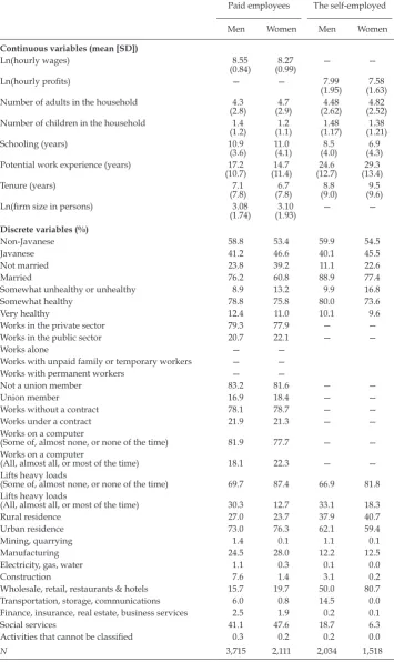
Appendix table A3 presents descriptive statistics that are similar to those from

other sources (Van Klaveren et al. 2010, for example). Two points are worth not

-ing. First, men and women, whether paid employees or self-employed, share sim

-ilar characteristics. This inding anticipates that characteristics play a small role in

(10)

explaining the gender gap. Admittedly, the marriage rate among paid employees

is smaller for women (60.8%) than for men (76.2%), which is consistent with the anecdotal evidence that many women are dismissed upon marriage or childbirth and that manufacturing industries prefer to hire young women (ADB 2006, 15). Men, whether paid employees or self-employed, are more likely than women to engage in jobs that require lifting heavy loads. However, it is shown below that these differences are not great enough to inluence the gender gap. Second, as many as 80.7% of self-employed women are engaged in the wholesale, retail, and restaurants and hotels sectors, whereas 50.0% of self-employed men are engaged in these sectors. Although not deinitive, this gives the impression of crowding

out.

Appendix igure A1 presents the distribution of earnings by sector and gender. In both sectors, the density curve for women is to the left of that of men, indicat

-ing that, on average, women earn less than men. However, when the two sec -tors are compared, the density curve for paid employees is slightly to the right of that for the self-employed for both genders, indicating that, on average, paid

employees earn more than the self-employed. This is consistent with the ind -ing that, in develop-ing countries, private-sector employment is considered to be

better than self-employment (Banerjee and Dulo 2011, chapter 9). In addition, the density curve is much wider for the self-employed than for paid employees

for both genders, a result commonly found in the literature on self-employment

(Parker 2009, chapter 13). The Indonesian labour market is typical for a develop

-ing country, and this opens the possibility that these ind-ings can be generalised

to other developing countries.

Paid Employees Earnings Regression

Table 1 presents the results estimated from speciication (1) with different sets of

characteristics. In column 1, only FEMALE is included in the speciication for the raw gap in earnings. The coeficient indicates that women earn 27% (e–0.315_{– 1)}

less than men. The size is similar to the mean of the raw wage gap in studies pub

-lished in the 1990s: 30% (Weichselbaumer and Winter-Ebmer 2005, 485). When the basic demographic variables are added to the speciication (column 2), the gap decreases slightly, to 22%. When the variables measuring human capital are also entered (column 3), the gap decreases, but again only slightly, to 19%. When the full set of characteristics is controlled for (column 4), the gap hardly changes, at 20%. Although speciic values vary depending on the set of characteristics entered,

the estimates of β1 do not differ statistically signiicantly from each other across

columns. The small effect of the characteristics on β1 beyond column 2 anticipates

that the gap in the decomposition at the mean is largely unexplained.

This small effect does not mean that the characteristics are irrelevant to

earn-ings. In fact, the size and sign of each coeficient make sense. According to column 4, married workers earn 7.4% more than unmarried ones, which is conceptualised

as the marriage premium in labour economics. An additional year of schooling is

associated with a 10% increase in wages, which is almost identical to the size that Sohn (2013) estimates using IFLS4. In addition, potential work experiences and tenure exhibit the usual inverse U-shaped relation to wages (Mincer 1974). Fur

(11)

TABLE 1 Gender Gap in Earnings in OLS: Paid Employees

(1) (2) (3) (4)

Female –0.315

(0.025)*** –0.250(0.030)*** –0.211(0.024)*** –0.219(0.022)***

Javanese –0.149

(0.063)** –0.149(0.039)*** (0.033)0.049

Married 0.380

(0.034)*** (0.033)***0.103 (0.028)**0.071

Somewhat healthy 0.064

(0.052) (0.039)0.042 (0.043)0.060

Very healthy 0.089

(0.099) (0.060)0.037 (0.062)0.081 No. of adults in household (/10) –0.072

(0.050) –0.159(0.046)*** –0.115(0.036)*** No. of children in household (/10) –0.060

(0.146) (0.097)0.133 (0.088)0.128

Schooling (years) 0.131

(0.006)*** (0.005)***0.099

Work experience (years) 0.020

(0.005)*** (0.004)***0.024 Work experience (years)2 (/100) _–0.019

(0.010)* –0.026(0.009)***

Tenure (years) 0.029

(0.004)*** (0.003)***0.019

Tenure (years)2 (/100) _–0.024

(0.012)** –0.012(0.010)

Works in the public sector 0.248

(0.039)***

Ln(irm size) 0.065

(0.005)***

Union member 0.161

(0.026)***

Works under a contract 0.103

(0.026)***

Works on a computer 0.231

(0.027)***

Lifts heavy loads –0.025

(0.028)

Urban residence 0.034

(0.039)

Constant 8.55

(0.04)*** (0.06)***8.30 (0.10)***6.66 (0.20)***7.63

9 industry ixed effects No No No Yes

20 province ixed effects No No No Yes

R2 _0.027 _0.066 _0.415 _0.500

Note: The sample size is 5,826. Sampling weights are applied. Standard errors clustered at the

sub-district level are in parentheses.

(12)

in this sector enjoy in developing countries (Banerjee and Dulo 2011, chapter 9). High-quality jobs, indicated by large irm size, union membership, working under a contract, and working on a computer, are all associated with greater earnings. It is also worth noting that the R2_{statistic is 0.500, which is greater than usual. Thus,}

the fact that these characteristics do not greatly reduce β1 implies that there is a

non-negligible amount of pay discrimination against women in Indonesia.

Decomposition at the Mean

Table 2 lists the results of decomposition at the mean with the full set of charac

-teristics (that is, those in column 4 of table 1). The decomposition is carried out in three ways, with different reference groups. In column 1, the male group is considered to be the reference group, meaning that the male coeficients and the female characteristics are used to estimate the counterfactual earnings of women. In column 2, the coeficients estimated in the pooled sample are used to estimate the counterfactual, as proposed by Neumark (1988), while the male and female coeficients are equally weighted for column 3, as proposed by Reimers (1983). The raw gap in column 1 of table 1 is repeated in the ‘Total gap’ row, with the

sign reversed, for reference purposes. Overall, the unexplained gap accounts for

about 70% of the raw gap, regardless of the reference group, and this proportion is similar to that found in the literature (for example, Meng 1998, for China; Liu 2004, for Vietnam; Menon and Rodgers 2009, for India). Since the irst method is conventional, the subsequent discussion focuses on column 1.

When the explained and unexplained gaps are further decomposed into gaps due to demographic controls, human capital, and job characteristics, more inter-esting results arise. The further decomposition for the explained gap indicates

that men have better demographics and more human capital than women. These variables, however, play a small role in the total gap because the unexplained gap dominates. Unfortunately, it is dificult to ind the detailed group of character -istics responsible for the unexplained gap, because, individually, the groups do

not have a statistically signiicant effect—despite having a signiicant effect when

considered collectively. The unconditional decomposition across the distribution,

below, addresses this puzzle. If coeficient size provides a guide to understand -ing the unexplained gap, one can see that human capital, job characteristics, and

the constant all play a signiicant role relative to the total gap, though in opposite

directions. While the total gap is 32 log points, the unexplained gap is –20 log

points owing to human capital, 17 log points owing to job characteristics, and 23 log points owing to the constant. In addition, the message delivered by the return to human capital is of some interest. These returns are higher for women than for men, which suggests that female paid employees are not always subject to discrimination. This argument is only tentative for now, but the unconditional

decomposition across the distribution yields richer evidence.

Decomposition across the Earnings Distribution

In the previous subsection, the gender gap in earnings is decomposed at the mean. This type of decomposition provides a good summary of the gap, but may hide more than it reveals. For example, the mean decomposition does not indicate

(13)

106 Kitae Sohn

Oaxaca decomposition to the entire distribution, conditional on characteristics;

this article employs the technique proposed by Chernozhukov, Fernández-Val, and Melly (2013). Their method addresses problems inherent in the compet

-ing approaches and is relatively lexible (Fortin, Lemieux, and Firpo, 2011, for details). Consistent with the convention, the male coeficients are treated as nor -mal. Because the sample sizes at both ends of the distribution are small, the range

of the distribution is restricted from quantiles 0.1 to 0.9.

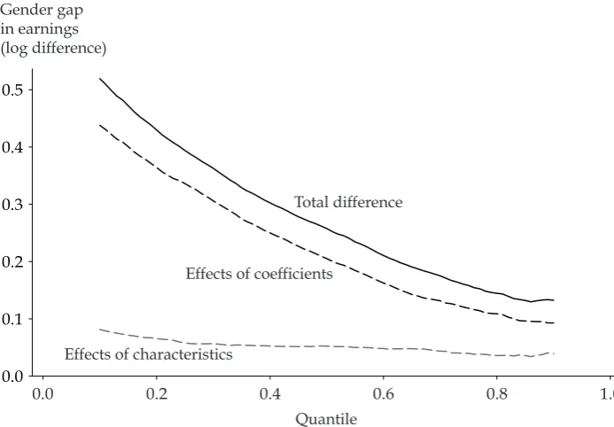
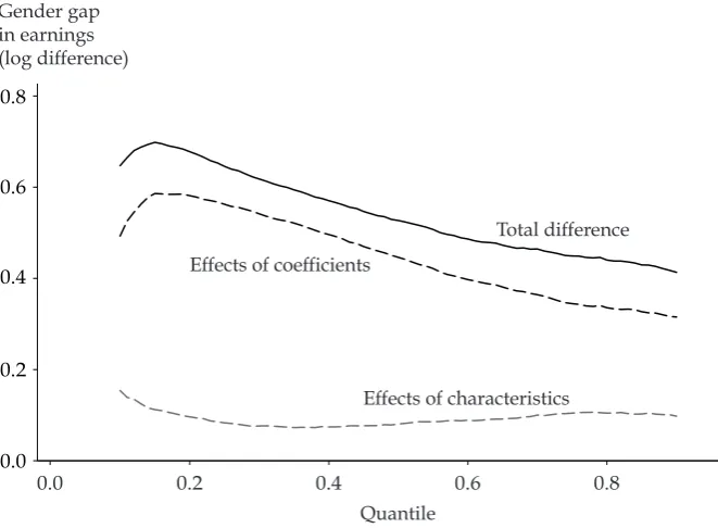
Figure 1 demonstrates that the total gap is much larger for low-earning women and monotonically declines as we move up the earnings distribution. Hence, the gap at quantile 0.1 is about 50 log points, while it is only about 10 log points at quantile 0.9. The explained gap is similar across the distribution. Therefore, the unexplained gap drives the total gap—the unexplained gap is statistically signii

-cant (appendix igure A2). Hence, it is dificult to account for the gap across the

earnings distribution, despite the large number of characteristics considered. In

addition, the downward trend in the unexplained gap (as we move up the earn

-ings ladder) suggests that the glass-ceiling effect for women is weak—otherwise,

TABLE 2 Decomposition of the Gender Gap in Earnings at the Mean: Paid Employees

Male

Note: The same covariates as in column 4 of table 1 are controlled for. The sample size is 5,826. Sam-pling weights are applied. Standard errors clustered at the sub-district level are in parentheses.

(14)

we would observe an upward trend. Thus, gender discrimination does not appear to be the main culprit for the small proportion of women in high positions and

among high-income earners.

Figure 1 displays the gender gap in the earnings distribution conditional on

characteristics; therefore, earnings at a certain quantile are decomposed for men and women who share the same characteristics. Firpo, Fortin, and Lemieux (2009) proposed another way of decomposing earnings at a certain quantile for men and women who do not necessarily share the same characteristics; this decomposition is based on unconditional quantile regressions. This is more intuitive than the conditional method, because it captures how people casually perceive the gender gap in earnings—they simply compare high-earning women and men, regardless

of their characteristics. I also provide detailed decomposition results. For

consist-ency, the male coeficients are treated as normal, and the analysis is restricted from quantiles 0.1 to 0.9.

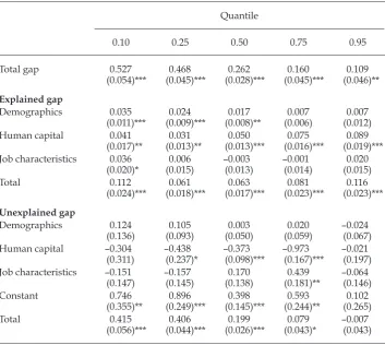
Table 3 shows that these results are similar to those obtained with the condi

-tional approach. As we move up the earnings distribution, the total gap decreases

from 53 log points to 11. The explained gap remains similar across the distribu-tion, and, therefore, the decrease in the unexplained gap primarily drives the decrease in the total gap.

These results help us to understand why human capital, job characteristics, and the constant all have statistically insigniicant effects on the size of the unexplained

gap. For example, in table 2, the size of the unexplained gap due to human capital

is large but statistically insigniicant; table 3 suggests that this is because the effect

FIGURE 1 Decomposition of the Gender Gap across the Earnings Distribution, Conditional on Characteristics: Paid Employees

0.0

Total difference

Effects of characteristics

Effects of coefficients

0.1 0.2 0.3 0.4 0.5 Gender gap in earnings (log difference)

Quantile

0.0 0.2 0.4 0.6 0.8 1.0

(15)

108 Kitae Sohn

is concentrated in the middle of the distribution. A similar explanation applies to the effect of job characteristics on the size of the unexplained gap. A more subtle

inding is that the returns to job characteristics can be higher or lower for women

than for men, depending on their positions in the distribution. The unexplained

gap due to the constant is also large but statistically insigniicant, as seen in table

2; table 3 suggests that this is because the effect is small in the upper part of the distribution. The constant plays the major role in accounting for the unexplained gap in tables 2 and 3. Since the constant contains ‘everything else’, this makes it

dificult to identify the responsible factors.

Self-Employed Workers Earnings Regression

Although the amount of paid work has grown as the Indonesian economy has

industrialised, the self-employed still account for more than half of the total TABLE 3 Decomposition of the Gender Gap across the Earnings Distribution,

Unconditional on Characteristics: Paid Employees

Quantile

0.10 0.25 0.50 0.75 0.95

Total gap 0.527

(0.054)*** (0.045)***0.468 (0.028)***0.262 (0.045)***0.160 (0.046)**0.109 Explained gap

Demographics 0.035

(0.011)*** (0.009)***0.024 (0.008)**0.017 (0.006)0.007 (0.012)0.007

Human capital 0.041

(0.017)** (0.013)**0.031 (0.013)***0.050 (0.016)***0.075 (0.019)***0.089 Job characteristics 0.036

(0.020)* (0.015)0.006 –0.003(0.013) –0.001(0.014) (0.015)0.020

Total 0.112

(0.024)*** (0.018)***0.061 (0.017)***0.063 (0.023)***0.081 (0.023)***0.116 Unexplained gap

Demographics 0.124

(0.136) (0.093)0.105 (0.050)0.003 (0.059)0.020 –0.024(0.067)

Human capital –0.304

(0.311) –0.438(0.237)* –0.373(0.098)*** –0.973(0.167)*** –0.021(0.197) Job characteristics –0.151

(0.147) –0.157(0.145) (0.138)0.170 (0.181)**0.439 –0.064(0.146)

Constant 0.746

(0.355)** (0.249)***0.896 (0.145)***0.398 (0.244)**0.593 (0.265)0.102

Total 0.415

(0.056)*** (0.044)***0.406 (0.026)***0.199 (0.043)*0.079 –0.007(0.043)

(16)

workforce. In this light, it is surprising that relatively little attention has been paid

to the self-employed in the literature.

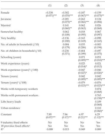
Table 4 reveals some interesting aspects of the gap in the sector. Column 1 shows the total gap, which indicates that self-employed women earned 29% less than self-employed men. This is similar to that for paid employees (27%). As more characteristics are added, the gap decreases to 15% in column 4. This column is

interesting in itself, because little research has been done on self-employment in

developing countries—for example, in Parker’s (2009) comprehensive textbook, it is dificult to ind references related to developing countries. Some characteristics that are relevant to wages are no longer relevant to proits. For example, marital status is no longer statistically signiicant. The return to schooling is just about half that for paid employees. Potential work experience does not appear to be important, but the association between tenure and proits is twice as great as that between tenure and wages. It seems that the earnings of the self-employed are

determined by different factors than those driving paid employees’ earnings, and

it is more dificult to ind the determinants of the earnings of the self-employed.

Decomposition at the Mean

Table 5 presents the decomposition results at the mean. As before, the ‘Total gap’

row indicates the value of β1 in column 1 of table 4, with the sign reversed. The

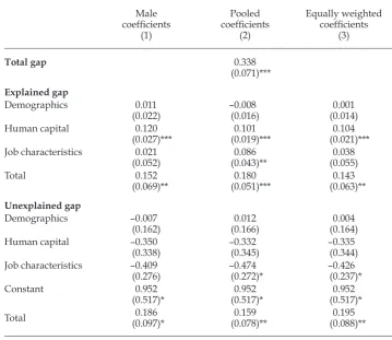
reference coeficients are constructed using the three methods mentioned above, but the patterns are similar regardless of the methods used. When the results with the male coeficients are considered, the explained and the unexplained gaps each account for about half of the total gap. This inding differs from that for paid employees, for whom the unexplained gap accounts for about three-quarters of the total gap. Recall that the total gap is similar between paid employees and the employed. Thus, it appears that women face less discrimination in self-employment than in paid work. However, the decomposition across the distribu

-tion, considered below, presents a more pessimistic picture.

One source of the gap for the self-employed is the higher human-capital

lev-els for men. This is consistent with the gap for paid employees. However, the explained gap due to human capital for self-employment is twice as great as that for paid work. Thus, according to column 1 of table 5, the gap due to gender

differences in human capital accounts for about a third of the total gap.

Further-more, none of the detailed groups individually has a statistically signiicant effect on the unexplained gap. However, they do have a statistically signiicant effect when considered collectively (their effect on the total unexplained gap is weakly signiicant at a p-value of 0.54 but signiicant using the other two methods). These results are similar to those for paid employees. As before, we can pay attention, for the moment, to the size rather than to the statistical signiicance (the results from the unconditional decomposition across the distribution will eventually explain much). The returns to human capital are higher for women than for men, which is consistent with the results for paid employees. However, the returns to job characteristics in self-employment are higher for women than for men, which

is in contrast to the corresponding results for paid employees. In addition, the unexplained gap due to the constant is substantially larger than in the case of

(17)

TABLE 4 Gender Gap in Earnings in OLS: The Self-Employed

(1) (2) (3) (4)

Female –0.338

(0.071)*** –0.302(0.070)*** –0.187(0.067)*** –0.159(0.075)**

Javanese –0.201

(0.075)** –0.262(0.066)*** (0.084)0.124

Married 0.141

(0.060)** (0.063)0.062 (0.068)0.026

Somewhat healthy 0.062

(0.108) (0.095)0.018 (0.097)0.067

Very healthy –0.136

(0.180) –0.163(0.169) –0.098(0.165) No. of adults in household (/10) 0.004

(0.179) (0.206)0.035 –0.003(0.194) No. of children in household (/10) –0.236

(0.371) –0.464(0.399) –0.497(0.375)

Schooling (years) 0.071

(0.009)*** (0.010)***0.051

Work experience (years) 0.023

(0.014)* (0.013)0.021 Work experience (years)2 (/100) _–0.047

(0.027)* –0.046(0.026)*

Tenure (years) 0.042

(0.009)** (0.009)***0.042

Tenure (years)2 (/100) _–0.079

(0.023)*** –0.076(0.023)***

Works with temporary workers 0.074

(0.068)

Works with permanent workers 0.765

(0.158)***

Lifts heavy loads 0.109

(0.068)

Urban residence 0.110

(0.060)*

Constant 7.89

(0.07)*** (0.17)***7.86 (0.21)***6.97 (1.12)***6.29

9 industry ixed effects No No No Yes

18 province ixed effectsa _No _No _No _Yes

R2 _0.008 _0.013 _0.049 _0.089

Note: The sample size is 3,552. Sampling weights are applied. Standard errors clustered at the

sub-district level are in parentheses.

a_{Two provinces have three and four observations for each, and, along with other dummy variables,} cause multicollinearity.

(18)

unexplained gap due to the constant favours men by 95 log points, resulting in a higher unexplained gap in favour of men. Hence, despite the favourable returns

to human capital and job characteristics, women in self-employment are still sub

-ject to an unfavourable gap stemming from unknowns.

Decomposition across the Earnings Distribution

Figure 2 shows the decomposition of the gender gap across the earnings distribu -tion. The general patterns are similar to those for paid employees. The total gap

decreases with earnings, and the unexplained gap drives the total gap across the distribution. In addition, the unexplained gap is statistically signiicant across the distribution (appendix igure A3). However, there is an important difference: the slopes of the total and unexplained gaps are latter than those for paid employ

-ees. Speciically, the total gap for the self-employed decreases from about 70 log points at quantile 0.1 to about 40 log points at quantile 0.9 (versus 50 to 10 log points for paid employees), and the unexplained gap is in parallel to the total gap.

TABLE 5 Decomposition of the Gender Gap in Earnings at the Mean: The Self-Employed

Male coeficients

(1)

Pooled coeficients

(2)

Equally weighted coeficients

(3)

Total gap 0.338

(0.071)*** Explained gap

Demographics 0.011

(0.022) –0.008(0.016) (0.014)0.001

Human capital 0.120

(0.027)*** (0.019)***0.101 (0.021)***0.104 Job characteristics 0.021

(0.052) (0.043)**0.086 (0.055)0.038

Total 0.152

(0.069)** (0.051)***0.180 (0.063)**0.143 Unexplained gap

Demographics –0.007

(0.162) (0.166)0.012 (0.164)0.004

(0.338) –0.332(0.345) –0.335(0.344) Job characteristics –0.409

(0.276) –0.474(0.272)* –0.426(0.237)*

Constant 0.952

(0.517)* (0.517)*0.952 (0.517)*0.952

Total _(0.097)*0.186 _(0.078)**0.159 _(0.088)**0.195

(19)

112 Kitae Sohn

Thus, when the gap is decomposed across the distribution, the unexplained gap

is greater than that for paid employees. Recall that according to the decomposi-tion at the mean, the unexplained gap is larger for paid employees than for the self-employed. The main reason for the contrasting results is that extreme values

of earnings (that is, those outside the quantiles 0.1–0.9; see also appendix igure A1) are taken into account for the mean decomposition but not for the distribution

decomposition. One can deduce from these that the unexplained gap is

consider-ably smaller—or even reversed in favour of women—for extreme values of earn

-ings, and the curved lines around quantile 0.1 suggest that the extremely low

values are the culprit.

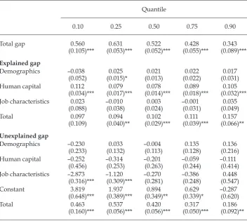
When the total gap is decomposed unconditional on characteristics (table 6),

the broad patterns in the results are similar to those obtained using the conditional

approach. In general, the total gap decreases as we move up the distribution, from 56 log points to 34. In addition, the results are consistent with and improve on the results derived from the Oaxaca decomposition (table 5). For example, table 5 shows that men’s having more human capital than women accounts for a large amount of the explained gap; table 6 shows that the relative importance increases with earnings. In addition, table 5 shows that the returns to job characteristics are higher for women than for men, although weakly or insigniicantly; table 6 shows that this favourable treatment is concentrated at the lower parts of the distribu

-tion. Similarly, table 5 shows that ‘everything else’, represented by the constant, accounts for a large amount of the unexplained gap; table 6 shows that this effect is largely concentrated at the lower parts of the distribution.

FIGURE 2 Decomposition of the Gender Gap across the Earnings Distribution, Conditional on Characteristics: The Self-Employed

0.0

Total difference

Effects of characteristics Effects of coefficients

0.2 0.4 0.6 0.8 Gender gap in earnings (log difference)

Quantile

0.0 0.2 0.4 0.6 0.8 1.0

(20)

It is of interest to compare these results with those for paid employees (table 3). The total gap for the self-employed decreases with earnings but not as dramati

-cally as the total gap for paid employees (from 53 to 11 log points). However, in

both sectors, human capital plays some role in the explained gap. In addition, the

higher returns to human capital for women than for men account for much of the

unexplained gap for paid employees in the middle of the earnings distribution, but this is not true for the self-employed. The job characteristics exert ambigu-ous effects on paid employees but discernible effects on the self-employed in the

lower parts of the distribution. However, the constant often exerts large effects in all parts (except for the upper ends) of the distribution, in both sectors.

CONCLUSIONS

The gender gap in earnings has been extensively studied in economics in the

context of discrimination. However, relatively little light has been shed on the gender gap in developing countries. Even when developing countries have been

TABLE 6 Decomposition of the Gender Gap across the Earnings Distribution, Unconditional on Characteristics: The Self-Employed

Quantile

0.10 0.25 0.50 0.75 0.90

Total gap 0.560

(0.105)*** (0.053)***0.631 (0.052)***0.522 (0.055)***0.428 (0.089)***0.343 Explained gap

(0.052) (0.015)*0.025 (0.013)0.021 (0.022)0.022 (0.031)0.017

Human capital 0.112

(0.034)*** (0.017)***0.079 (0.014)***0.078 (0.018)***0.089 (0.032)***0.105 Job characteristics 0.023

(0.088) –0.010(0.038) (0.024)0.003 –0.001(0.031) (0.049)0.035

Total 0.097

(0.109) (0.040)**0.094 (0.029)***0.102 (0.039)***0.111 (0.066)**0.157 Unexplained gap

(0.233) (0.132)0.033 –0.004(0.113) (0.128)0.135 (0.216)0.136

(0.456) –0.314(0.253) –0.201(0.263) –0.059(0.244) –0.111(0.414) Job characteristics –2.873

(0.316)*** –1.120(0.309)*** –0.270(0.281) –0.386(0.248) (0.547)0.448

Constant 3.819

(0.648)*** (0.389)***1.937 (0.349)**0.894 (0.339)*0.629 –0.287(0.620)

Total 0.463

(0.160)*** (0.056)***0.537 (0.056)***0.420 (0.050)***0.317 (0.092)**0.186

(21)

114 Kitae Sohn

considered, decomposition has been performed at the mean of earnings, which can hide more than it reveals about the dynamics of discrimination. Moreover,

despite the large number of the self-employed in the labour force in developing countries, the literature has generally neglected them. This article analyses data from IFLS4 in order to assess discrimination among paid employees and the self-employed, not only at the mean of earnings but also across the entire distribution.

The workhorse econometric method used is the Oaxaca decomposition and its extensions to quantile regressions; for the extensions, characteristics are both con -ditioned and uncon-ditioned.

Women earned about 30% less than men in both paid work and self-employment. Differences in characteristics account for only about a quarter of the gap in paid work

but for about half of the gap in self-employment. In particular, differences in human

capital play an important role in explaining the gap in self-employment. At irst

glance, this suggests that the self-employed are less subject to gender discrimination than paid employees, but the decomposition across the distribution contradicts this. It appears that the competition generated by more than four decades of sustained

economic growth did not substantially reduce discrimination in paid work and self-employment. Menon and Rodgers (2009) reported similar indings for India. My results suggest that Becker’s (1957) theory is not plausible for Indonesia. This does not automatically support Rosén’s (2003) theory, but it is worth considering.

When the decomposition is made across the distribution of earnings, the total

gap decreases with earnings for both paid work and self-employment and is

both conditional and unconditional on characteristics. In both sectors, the gap due to differences in characteristics remains similar across the distribution, and therefore the decrease in the unexplained gap drives the decrease in the total gap. The decrease is steeper for paid employees than for the self-employed, so the unexplained gap in the upper parts of the distribution is relatively small for paid employees. It seems that the glass-ceiling effect is not strong in Indonesia. On the other hand, the level of the unexplained gap is higher for the self-employed than for paid employees across the distribution. This suggests that discrimination

against self-employed women is pervasive.

The unconditional decomposition in the earnings distribution provides great insight into the dynamics obscured in the results derived from the decomposi-tion at the mean. When the gap is decomposed at the mean, none of the

indi-vidual groups has a signiicant effect on the unexplained gap (in either sector), but the collective effect is signiicant. The unconditional decomposition across the distribution explains this; some effects may be strong or weak and even change

direction, depending on their positions in the earnings distribution. In addition,

in paid work, the returns to human capital are higher for women than for men in

the middle of the distribution. On the other hand, in self-employment, the returns

to job characteristics are higher for women than for men in the lower parts of the distribution. Hence, Indonesian women do experience favourable treatment for

some characteristics. That said, the unexplained gap due to the constant is large in both sectors, implying that much of the unexplained gap remains unexplained. This is the main limitation of this article, and I hope that future research can iden-tify factors that account for this large unexplained gap.

(22)

my evidence is only suggestive. However, three points imply that the existence

of discrimination is not implausible. First, a substantial proportion of the

unex-plained gap remains, even when a large number of characteristics are accounted for. Second, women in the sample are likely to possess higher abilities than men,

on average. Third, the decomposition conditional and unconditional on charac-teristics yields similar results.

If there is indeed substantial discrimination against women in the labour mar

-ket, what drives it? I do not have deinitive evidence, but I can speculate that it

is largely driven by the cultural, religious, and social norms in Indonesia

men-tioned in ‘The Indonesian Context’, above. A more interesting point is how these norms are differentially applied. The great discrimination against low-earning women in paid employment may be generated by employers who believe that women are less attached than men to the labour market, so these employers offer more opportunities for earnings growth to men than to women. Experiencing or anticipating this, women may be discouraged from pursuing greater earnings. On the other hand, the low level of discrimination against high-earning women

in paid employment suggests that employers do not base their personnel deci-sions on these ideologies—possibly because they understand that high-earning

women face a high opportunity cost when staying at home and that these women

are therefore strongly attached to the labour market. Experiencing or

anticipat-ing this, high-earnanticipat-ing women may behave as expected. In contrast, the more or less constant discrimination against women in self-employment may be driven by customers. Customers may believe that women in some sectors do not produce quality goods, or customers may not buy certain goods if they are made or sold by women. In this case, women with the appropriate skills can be discouraged from

joining the sectors. Because this belief is related not to the labour-market

attach-ment but to women’s (putatively) inherent skills, discrimination based on this belief can affect both low- and high-earning women in self-employment. Recall that 81% of women in self-employment work in the wholesale, retail, and restau

-rants and hotels sectors, which are close to the domestic sphere.

This article demonstrates the beneits of decomposing the gender gap across the earnings distribution; the rich dynamics uncovered by this method warn

against relying only on decomposition at the mean. As my previous studies (Sohn

2012a, 2012b, 2014) have shown, similar econometric strategies can provide new

insights into outcomes other than gender earnings gaps, using both contempo-rary and historical data.

As for policy-making, this article illustrates how to identify target groups more

precisely. It may be a policy priority to target the groups that suffer from a large gender earnings gap due to discrimination; my results indicate that, in Indonesia,

this group comprises low-earning women in both paid work and self-employ -ment. Yet policymakers need to remember that the returns to some characteristics are lower for men than for women, depending on the individual’s position in the earnings distribution. This implies that indiscriminately promoting treatments

favouring women may unintentionally hurt some groups of men.

Before concluding, I wish to suggest a future research topic. Recall that although

the IFLS comprises longitudinal data, this study employs cross-sectional data.

(23)

116 Kitae Sohn

gender gap in earnings in Indonesia. Bertrand, Goldin, and Katz’s (2010) study is

a good example of such an effort. The critical strength of their study is their

track-ing a homogeneous group (MBAs who graduated between 1990 and 2006 from a top US business school) up to 16 years after graduation, which allowed them to

control for many unobservable characteristics. The IFLS is not suitable for such an exercise, but the idea itself can contribute to our understanding of career

dynam-ics by gender, particularly for high earners in Indonesia. Utomo (2008) provided

a promising lead.

REFERENCES

ADB (Asian Development Bank). 2006. Country Gender Assessment: Indonesia. Manila: ADB. Akerlof, George A., and Rachel E. Kranton. 2010. Identify Economics: How Our Identities

Shape Our Work, Wages, and Well-Being. Princeton: Princeton University Press.

Banerjee, Abhijit V., and Esther Dulo. 2011. Poor Economics: A Radical Rethinking of the Way to Fight Global Poverty. New York: Public Affairs.

Becker, Gary. 1957. The Economics of Discrimination. Chicago: Chicago University Press. Benjamin, Dwyne. 1996. ‘Women and the Labour Market in Indonesia during the 1980s’.

In Women and Industrialization in Asia, edited by Susan Horton, 81–133. London: Rout-ledge.

Bergmann, Barbara R. 1971. ‘The Effect on White Incomes of Discrimination in Employ-ment’. Journal of Political Economy 79 (2): 294–313.

Bertrand, Marianne, Claudia Goldin, and Lawrence F. Katz. 2010. ‘Dynamics of the Gender Gap for Young Professionals in the Financial and Corporate Sectors’. American Economic Journal: Applied Economics 2 (3): 228–55.

Blinder, Alan S. 1973. ‘Wage Discrimination: Reduced Form and Structural Estimates’. Jour-nal of Human Resources 8 (4): 436–55.

Byron, R. P., and H. Takahashi. 1989. ‘An Analysis of the Effect of Schooling, Experience and Sex on Earnings in the Government and Private Sectors of Urban Java’. Bulletin of Indonesian Economic Studies 25 (1): 105–17.

Chernozhukov, Victor, Iván Fernández-Val, and Blaise Melly. 2013. ‘Inference on Counter -factual Distributions’. Econometrica 81 (6): 2205–68.

Deolalikar, Anil B. 1993. ‘Gender Differences in the Returns to Schooling and in School Enrolment Rates in Indonesia’. Journal of Human Resources 28 (4): 899–932.

Firpo, Sergio, Nicole M. Fortin, and Thomas Lemieux. 2009. ‘Unconditional Quantile Regressions’. Econometrica 77 (3): 953–73.

Fortin, Nicole, Thomas Lemieux, and Sergio Firpo. 2011. ‘Decomposition Methods in Eco -nomics’. In Handbook of Labor Economics, vol. 4, edited by Orley Ashenfelter and David Card, 1–102. Amsterdam: North-Holland.

Goldin, Claudia. 1990. Understanding the Gender Gap: An Economic History of American Women. New York: Oxford University Press.

Hochschild, Arlie, and Anne Machung. 1989. The Second Shift: Working Parents and the Re volution at Home. New York: Viking Penguin.

Jones, F. L., and Jonathan Kelley. 1984. ‘Decomposing Differences between Groups: A Cau -tionary Note on Measuring Discrimination’. Sociological Methods and Research 12 (3): 323–43.

Liu, Amy Y. C. 2004. ‘Gender Wage Gap in Vietnam: 1993 to 1998’. Journal of Comparative Economics 32 (3): 586–96.

(24)

Menon, Nidhiya, and Yana van der Meulen Rodgers. 2009. ‘International Trade and the Gender Wage Gap: New Evidence from India’s Manufacturing Sector’. World Develop-ment 37 (5): 965–81.

Mincer, Jacob A. 1974. Schooling, Experience, and Earnings. Cambridge, MA: National Bureau of Economic Research.

Neumark, David. 1988. ‘Employers’ Discriminatory Behavior and the Estimation of Wage Discrimination’. Journal of Human Resources 23 (2): 279–95.

Oaxaca, Ronald. 1973. ‘Male-Female Wage Differentials in Urban Labour Markets’. Interna-tional Economic Review 14 (3): 693–709.

Parker, Simon C. 2009. The Economics of Entrepreneurship. Cambridge, UK: Cambridge Uni -versity Press.

Posner, Richard A. 1989. ‘An Economic Analysis of Sex Discrimination Laws’. University of Chicago Law Review 56 (4): 1311–35.

Reimers, Cordelia W. 1983. ‘Labor Market Discrimination against Hispanic and Black Men’. Review of Economics and Statistics 65 (4): 570–79.

Rosén, Åsa. 2003. ‘Search, Bargaining, and Employer Discrimination’. Journal of Labor Eco-nomics 21 (4): 807–29.

Setyonaluri, Diahhadi. 2014. ‘Women Interrupted: Determinants of Women’s Employment Exit and Return in Indonesia’. PhD diss. abstract. Bulletin of Indonesian Economic Studies 50 (3): 485–6.

Sohn, Kitae. 2012a. ‘The Dynamics of the Evolution of the Black-White Test Score Gap’. Education Economics 20 (2): 175–88.

———. 2012b. ‘A New Insight into the Gender Gap in Math’. Bulletin of Economic Research 64 (1): 135–55

———. 2013. ‘Monetary and Nonmonetary Returns to Education in Indonesia’. Developing Economies 51 (1): 34–59

———. 2014. ‘The Gender Gap in Earnings among Teachers: The Case of Iowa in 1915’. Fem -inist Economics. Published electronically 28 August. doi: 10.1080/13545701.2014.936481.

———. 2015. ‘The Height Premium in Indonesia’. Economics and Human Biology 16: 1–15. Utomo, Ariane J. 2008. ‘Women as Secondary Earners: The Labour Market and Mar

-riage Expectations of Educated Youth in Urban Indonesia’. PhD diss., The Australian National University.

Van der Eng, Pierre. 2010. ‘The Sources of Long-Term Economic Growth in Indonesia, 1880–2008’. Explorations in Economic History 47 (3): 294–309.

Van Klaveren, Maarten, Kea Tijdens, Melanie Hughie-Williams, and Nuria Ramos Martin. 2010. ‘An Overview of Women’s Work and Employment in Indonesia’. Working Paper 10-91, University of Amsterdam, Amsterdam.

(25)

118 Kitae Sohn

APPENDIX

Some Statistics on the Indonesian Labour Market

We can use IFLS4 to get an impression of the adverse conditions that women face in the Indonesian labour market. The sample is restricted to men and women aged 18–65, excluding those engaging in agriculture, forestry, ishing, and hunt

-ing. Here, I consider a broad deinition of labour-force participation. Speciically, an individual who meets any of the following criteria is considered to be partici

-pating in the labour market: (1) his or her primary activity during the past week was working, trying to work, or helping to earn income; (2) he or she worked tried to work, or helped to earn income for at least one hour during the past week; (3) he or she had a job or business but was temporarily not working during the past week; and (4) he or she worked at a family-owned (farm or non-farm) busi

-ness during the past week. As table A1 shows, 89.7% of men met any one of the criteria, but only 60.3% of women did; among non-working women, 89.6% said that their primary activity during the past week was housekeeping.

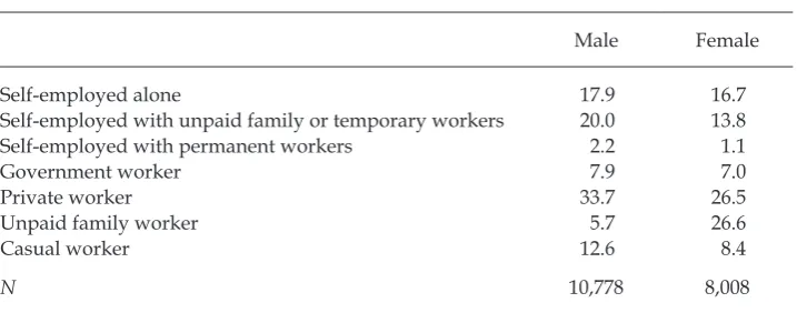
For working women, the quality of their employment was worse than that for men. Table A2 shows that 20.0% of men were self-employed with unpaid family or temporary workers, but only 13.8% of women were. Similarly, while 33.7% of men worked in the private sector, only 26.5% of women did. Private-sector work

is typically considered to be superior to self-employment in Indonesia; table A3

and igure A1 provide further evidence for this in terms of earnings. Even worse, 26.6% of women were unpaid family workers, compared with only 5.7% of men.

TABLE A1 Labour-Force Participation by Gender (%)

Male Female

Non-working 10.3 39.7

Working 89.7 60.3

N 12,017 13,274

TABLE A2 Employment Sector by Gender (%)

Male Female

Self-employed alone 17.9 16.7

Self-employed with unpaid family or temporary workers 20.0 13.8

Self-employed with permanent workers 2.2 1.1

Government worker 7.9 7.0

Private worker 33.7 26.5

Unpaid family worker 5.7 26.6

Casual worker 12.6 8.4

(26)

Paid employees The self-employed Number of adults in the household 4.3

(2.8) (2.9)4.7 (2.62)4.48 (2.52)4.82 Number of children in the household 1.4

(1.2) (1.1)1.2 (1.17)1.48 (1.21)1.38 Schooling (years) 10.9

(3.6) 11.0(4.1) (4.0)8.5 (4.3)6.9 Potential work experience (years) 17.2

(10.7) (11.4)14.7 (12.7)24.6 (13.4)29.3 Tenure (years) 7.1

Not married 23.8 39.2 11.1 22.6

Married 76.2 60.8 88.9 77.4 Somewhat unhealthy or unhealthy 8.9 13.2 9.9 16.8 Somewhat healthy 78.8 75.8 80.0 73.6

Very healthy 12.4 11.0 10.1 9.6

Works in the private sector 79.3 77.9 — —

Works in the public sector 20.7 22.1 — —

Works alone — —

Works with unpaid family or temporary workers — — Works with permanent workers — —

Not a union member 83.2 81.6 — —

Union member 16.9 18.4 — —

Works without a contract 78.1 78.7 — —

Works under a contract 21.9 21.3 — —

Works on a computer

(Some of, almost none, or none of the time) 81.9 77.7 — — Works on a computer

(All, almost all, or most of the time) 18.1 22.3 — — Lifts heavy loads

(Some of, almost none, or none of the time) 69.7 87.4 66.9 81.8 Lifts heavy loads

(All, almost all, or most of the time) 30.3 12.7 33.1 18.3

Rural residence 27.0 23.7 37.9 40.7

Urban residence 73.0 76.3 62.1 59.4

Mining, quarrying 1.4 0.1 1.1 0.1 Manufacturing 24.5 28.0 12.2 12.5 Electricity, gas, water 1.1 0.3 0.1 0.0 Construction 7.6 1.4 3.1 0.2 Wholesale, retail, restaurants & hotels 15.7 19.7 50.0 80.7 Transportation, storage, communications 6.0 0.8 14.5 0.0 Finance, insurance, real estate, business services 2.5 1.9 0.2 0.1

Social services 41.1 47.6 18.7 6.3

Activities that cannot be classiied 0.3 0.2 0.2 0.0

(27)

FIGURE A1 Earnings Distribution by Sector and Gender

0 0.0 0.1 0.2 0.3 0.4 0.5

5 10 15

0 5 10 15

Log of profits Log of wages

0.0 0.1 0.2 0.3 0.4

Male Female Density

Paid employees

The self-employed