Manajemen | Fakultas Ekonomi Universitas Maritim Raja Ali Haji 073500102288618874

Full Terms & Conditions of access and use can be found at

http://www.tandfonline.com/action/journalInformation?journalCode=ubes20

Download by: [Universitas Maritim Raja Ali Haji] Date: 13 January 2016, At: 00:39

Journal of Business & Economic Statistics

ISSN: 0735-0015 (Print) 1537-2707 (Online) Journal homepage: http://www.tandfonline.com/loi/ubes20

On Unit-Root Tests When the Alternative Is a

Trend-Break Stationary Process

Amit Sen

To cite this article: Amit Sen (2003) On Unit-Root Tests When the Alternative Is a Trend-Break Stationary Process, Journal of Business & Economic Statistics, 21:1, 174-184, DOI: 10.1198/073500102288618874

To link to this article: http://dx.doi.org/10.1198/073500102288618874

View supplementary material

Published online: 01 Jan 2012.

Submit your article to this journal

Article views: 61

View related articles

On Unit-Root Tests When the Alternative

Is a Trend-Break Stationary Process

Amit

Sen

Department of Economics & Human Resources, Xavier University, Cincinnati, OH 45207-3212 (sen@xavier.edu)

Minimumtstatistics to test for a unit-root are available when the form of break under the alternative evolves according to the crash, changing growth, and mixed models. It is shown that serious power distortions occur if the form of break is misspeciŽed, and thus the practitioner should use the mixed model as the appropriate alternative in empirical applications. The mixed model may reveal useful information regarding the location and form of break. The maximumF statistic for the joint null of a unit-root and no breaks is shown to have greater and less erratic power compared to the minimumt

statistic. Stronger evidence against the unit-root is found for the Nelson–Plosser series and U.S. Postwar quarterly real gross national product.

KEY WORDS: Break-date; Form of break; MaximumF statistic; Minimumtstatistic.

1. INTRODUCTION

Perron (1989) demonstrated that the conventional Dickey and Fuller (1979) t statistic (tDF) accepts the null

hypothe-sis of a unit-root far too often when the true data-generating process is in fact trend stationary with a break in the inter-cept or the slope of the trend function. Three different char-acterizations of the trend-break alternative were considered: (a) the crash model, which allows for a break in the intercept; (b) the changing growth model, which allows for a break in the slope with the two segments joined at the break-date; and (c) the mixed model, which allows for a simultaneous break in the intercept and the slope. To devise unit-root tests that have power against the trend-break stationary alternative, Per-ron (1989) proposed the following methodology: First spec-ify the location of the break-date (Tb), and then estimate a

regression that nests the random walk null and the trend-break stationary alternative of choice. Under the null hypothesis, Perron derived the limiting distribution of thetstatistic on the Žrst lag of the dependent variable, denoted byti

DF4Tb5, where

iDA, B, or C corresponds to the crash, the changing growth, or the mixed model, respectively. The limiting distribution of ti

DF4Tb5depends on the location and form of break under the

alternative hypothesis.

The assumption that the location of break is known a pri-ori was criticized by a number of studies, most notably by Christiano (1992). Also, see Banerjee, Lumsdaine, and Stock (1992), Zivot and Andrews (1992), and Perron and Vogelsang (1992). Christiano (1992) argued that the choice of the break-date is in most cases correlated with the data; for example, the practitioner may determine the location of the break-date by visually inspecting a plot of the time series. And because Perron’s (1989) methodology does not account for this ‘pretest examination of data,’ the unit-root null will be rejected too often. A number of studies proposed extensions for unit-root tests that do not require the practitioner to prespecify the location of break; see Zivot and Andrews (1992), Banerjee et al. (1992), Perron and Vogelsang (1992), Perron (1997), and Vogelsang and Perron (1998). The strategy adopted by these studies is to apply Perron’s (1989) methodology for each possible break-date in the sample, which yields a sequence of t statistics. Based on this sequence, numerous minimum tstatistics can be constructed by choosing thetstatistic, based

on some algorithm, that maximizes evidence against the null hypothesis. For example, one may simply use the minimum of the sequence oftstatistics, denoted bytmin

DF4i51 iDA, B, C.

With the availability of the minimumt statistics, the prac-titioner no longer needs to prespecify the location of break. However, one must still specify the form of break under the alternative hypothesis. If one assumes that the location of break is unknown, it is most likely that the form of break will be unknown as well. It is argued here that selection of the form of break is also correlated with the data and so one must pro-ceed with the break speciŽcation according to the most general mixed model. In addition, one may expect power distortions if the form of break is misspeciŽed, that is, if one imposes the crash (changing growth) model when in fact the changing growth (crash) or the mixed model is appropriate. Consider, for example, the use of the crash model speciŽcation under the alternative hypothesis when the break occurs according to the changing growth or the mixed model. The crash model minimumtstatistictmin

DF4A5is designed to maximize evidence

against the null hypothesis in favor of this particular alterna-tive. If the true data-generating process is given by the mixed model, the power of tmin

DF4A5 can be expected to be lower

than that of tmin

DF4C5, especially if the magnitude of the slope

break is relatively large. Even lower power oftmin

DF4A5may be

expected if the alternative evolves according to the changing growth model. On the other hand, if the crash hypothesis is the correct speciŽcation, then its use will yield superior power compared to the mixed model statistics. In practice, however, one is uncertain about the form of break. Because one would like to guard against distortions in power owing to misspeciŽ-cation of the form of break, it is recommended that the practi-tioner use the mixed model speciŽcation under the alternative hypothesis.

The Žrst objective is to assess the performance of minimum t statistics when the form of break is misspeciŽed. To this end, simulation evidence is provided (a) on the performance

©2003 American Statistical Association Journal of Business & Economic Statistics January 2003, Vol. 21, No. 1 DOI 10.1198/073500102288618874 174

of the crash model statistics when the break occurs according to either the changing growth or the mixed model; (b) on the performance of the changing growth model statistics when the break occurs according to either the crash or the mixed model; and (c) to assess the loss in power of the mixed model statis-tics when the break occurs according to either the crash or the changing growth model. It is found that the loss in power is quite small if the mixed model speciŽcation is used when in fact the break occurs according to the crash model. The loss in power is more substantial if the break occurs according to the changing growth model. However, serious distortions can occur if the crash (changing growth) model is used when the appropriate model is either the changing growth (crash) model or the mixed model. Therefore, the results indicate that one should use the form of the break speciŽed under the mixed model, unless prior information about the nature of the break suggests using either the crash model or the changing growth model. In most cases, it is expected that information on the form of break will be accompanied with information on the location of break, in which case Perron’s (1989) tests should be used. Also studied are the power properties the supWald (or equivalently the maximumF statistic, denoted byFmax

T )

pro-posed by Murray (1998) and Murray and Zivot (1998) for the joint null hypothesis of a unit-root and no break in the inter-cept and slope of the trend function. Simulation results show that the power ofFmax

T is less erratic and can be greater than

the mixed model minimumt statistics.

Second, the arguments are illustrated within the context of an empirical example that has received much attention in the literature. Numerous studies have used the Nelson and Plosser (1982) data and postwar quarterly real gross national product (GNP) to test for the presence of a unit-root. Per-ron (1989) speciŽed the great crash of 1929 as the break-date for all Nelson–Plosser series and the oil price shock of 1973 for quarterly real GNP. Conditional on these break-dates, the crash model was speciŽed for all Nelson–Plosser series except common stock prices and real wages, for which the mixed model was used, and the changing growth model was used for quarterly real GNP. Whereas subsequent studies by Zivot and Andrews (1992), Perron (1997), Nunes, Newbold, and Kuan (1997), and Murray and Nelson (2000) allowed for an unknown break-date, they retained the model speciŽcation proposed by Perron (1989). Unlike in these studies, empirical evidence is presented here for the presence of a unit-root in all series when the alternative allows for a simultaneous break in the intercept and slope. It is found that the unit-root null can be rejected for all series with the exception of the GNP deator, consumer prices, velocity, and interest rate series. The results are robust to possible misspeciŽcation of the form of break and therefore reveal useful information regarding the location and form of break. For instance, the empirical evidence of Zivot and Andrews (1992) indicates that real per capita GNP is characterized as a stationary process with break in the inter-cept occurring in 1929, and both money stock and quarterly real GNP contain a unit-root. By using the mixed model as the appropriate alternative, evidence is strengthened against a unit-root in real per capita GNP, and evidence is uncovered against the unit-root for money stock and quarterly real GNP. The break-date is estimated for real per capita GNP in 1938,

for money stock in 1930, and for quarterly real GNP in 1964, fourth quarter. The estimated break-dates for these series are different from the estimated break-dates reported by Zivot and Andrews (1992).

The outline of this article is as follows. Section 2 discusses the minimum t statistics and the maximum F statistic that have been proposed in the literature. In Section 3, simulation evidence is presented that enables one to study the Žnite sam-ple size and power properties of all statistics when the form of break may be misspeciŽed. Empirical evidence for the Nel-son and Plosser (1982) data and U.S. postwar quarterly real GNP is presented in Section 4. Concluding comments appear in Section 5.

2. TEST STATISTICS AND METHODOLOGY

We begin with a brief discussion of the null and alterna-tive hypotheses of interest, the class of minimum tstatistics, and the maximumF statistic. The discussion follows the anal-ysis by Zivot and Andrews (1992). Consider the time series 8yt9TtD1, whereT is the available sample size. The three

differ-ent characterizations of the alternative hypothesis, originally discussed by Perron (1989), are given by

Model (A)2 ytDŒ0CŒ1DUt4T

For the asymptotic results, it is assumed that the break-date is a constant fraction of the sample size, that is, Tc

b D‹cT

with the correct break-fraction‹c_{240115. It is assumed that}

A4L5etDB4L5t, andt is a sequence of iid401‘25random

variables, A(L) and B(L) are polynomials in the lag opera-tor of order pC1 and q, respectively, with all roots outside the unit circle. Model (A) is referred to as the crash model because it allows for a break in the intercept alone, Model (B) is referred to as the changing growth model because it allows for a break in the slope with the two segments joined at the break-date, and Model (C) is referred to as the mixed model because it allows for a simultaneous break in the intercept and the slope of the trend function.

The data-generating process given in (1)–(3), known as the additive outlier (AO) model, incorporates a break in the trend function that occurs instantaneously. This article considers the innovation outlier (IO) model, wherein the change in the trend function evolves in the same manner as any other shock; see section 4.2 in the work by Perron (1989). That is,

Model (A)2 ytDŒ0CŒ2tC–4L56Œ1DUt4Tbc5Ct71 (4)

where –4L5DA4L5ƒ1_{B4L5. The impact of the break is}

dif-ferent in the AO and IO models. Consider, for example, the

crash model speciŽcation of the break. In the AO characteri-zation, the magnitude of the break isŒ1. However, in the IO

characterization the immediate impact of the break is equal to Œ₁, but the long-run impact is equal to–415Œ₁.

Under the null hypothesis, the data-generating process con-tains a unit-root, that is,

y_tDŒCy_tƒ1C– ü

4L5_t1 (7)

where –ü_4L5DAü_4L5ƒ1_{B4L51 A4L5D41ƒL5A}ü_{4L5, and}

D1. To test for a unit-root in the IO framework, the fol-lowing methodology has been suggested. Specify an interval åD6‹011ƒ‹07 40115 that is believed to contain the true

break-fraction. For each possible‹2å, estimate the following regression that nests the null and the appropriate alternative:

ytD OŒA0C OŒ

where [.] is the smallest integer function. The additional k regressors8ãytƒj9kjD1 are included in the regression to

elim-inate the correlation in the disturbance term. Typically, the value of the lag-truncation parameter (k) is unknown, and so a data-dependent method for choosing the appropriate value of k is used; see Perron and Vogelsang (1992), Hall (1992, 1994), Perron (1997), and Ng and Perron (1995). We use Per-ron and Vogelsang’s (1992) data-dependent method k4t-sig) for selecting the lag-truncation parameter, which is described in what follows. Specify an upper bound k-max for the lag-truncation parameter. For each break-date6‹T 7, the cho-sen value of the lag-truncation parameter (kü_{) is determined}

according to the following general to speciŽc procedure: The last lag in an autoregression of order kü _{is signiŽcant, but}

the last lag in an autoregression of order greater than kü _is

insigniŽcant. The signiŽcance of the coefŽcient is assessed using the 10% critical values based on a standard normal dis-tribution. Regressions (8)–(10) are estimated for the break-dates 86‹0T 71 6‹0T 7C11 : : : 1 Tƒ6‹0T 79, and the sequence

of t statistics for H₀2  D1, denoted by 8ti DF4Tb59

Tƒ6‹₀T 7 TbD6‹0T 7

(iDA, B, C) is calculated. Based on this sequence, a number of minimum t statistics can be obtained by using an algo-rithm to choose the appropriate break-date that maximizes evi-dence against Equation (7); see Perron and Vogelsang (1992), Banerjee et al. (1992), Perron (1997), and Vogelsang and Perron (1998).

We consider two particular algorithms for choosing the break-date. The Žrst statistic, originally proposed by Perron and Vogelsang (1992) and Zivot and Andrews (1992), is obtained by choosing the break-date that maximizes evidence against the unit-root null, that is,

tmin

DF4i5DMinTb286‹0T 716‹0T 7C11 : : : 1Tƒ6‹0T 79t

i

DF4Tb5 (11)

foriDA, B, C. Perron (1997) demonstrated thattmin

DF4i5can be

calculated with åD40115so that no trimming of the sample is necessary. The second statistic, proposed by Banerjee et al. (1992) and Vogelsang and Perron (1998), is deŽned as

O

The minimumt statistics,tmin

DF4i5andOtDF4i5(iDA, B, C),

do not require speciŽcation of the location of break. However, the practitioner does need to specify the form of break under the alternative hypothesis. Once the break-date is treated as unknown, the practitioner will in most cases be unaware of the form of break. Because the crash and changing growth models are special cases of the mixed model, the practitioner should specify the mixed model as the appropriate alternative. Some loss in power can be expected from using the statistics from the mixed model when in fact the break occurs according to the crash or changing growth model. However, the behavior of the statistics from the crash (changing growth) model when the break occurs according to the changing growth (crash) or mixed model is uncertain. The next section presents simula-tion evidence regarding the power properties of the minimum t statistics when the form of break is misspeciŽed.

Next, we briey describe the supWald statistic proposed by Murray (1998) and Murray and Zivot (1998) for the joint null hypothesis of a unit-root and no break in the intercept and slope of the trend function. As before, it is assumed that the break-fraction lies in åD6‹011ƒ‹07. For each

possi-ble break-dateTb286‹0T 71 6‹0T 7C11 : : : 1 Tƒ6‹0T 79, theF

statistic, denoted by F_T4T_b5 from regression (10) that corre-sponds to the joint null hypothesisHJ

02 D11 Œ1D0,Œ3D0

where Œ4TO b5 is the ordinary least squares (OLS) estimator

ofŒD4Œ01 Œ11 Œ21 Œ31 1 c11 : : : 1 ck5 number of restrictions, ‘O2_4T

b5 D4T ƒ5ƒk5

ƒ1PT tD14ytƒ

x_t4T_b50_Œ4TO

b552, andR is deŽned so thatRŒDr corresponds

to the restrictions imposed on the parameter vectorΠby the joint nullHJ

Table 1. Critical Values forFmax

T WithåD[‹0,1-‹0]

1% 2.5% 5% 10%

‹0D015

TD50 kD0 1301238 1106071 1005840 904661

k(t-sig) 1500101 1302783 1202464 1008523

TD100 kD0 1200157 1008744 1000248 900628

k(t-sig) 1300842 1108875 1007809 907820

TD150 kD0 1108505 1007593 909333 809723

k(t-sig) 1208437 1102872 1003951 904935

TD200 kD0 1106450 1004785 906730 808708

k(t-sig) 1206811 1100691 1003038 903692

TD ˆ 1009288 1001691 904376 806958

‹0D010

TD50 kD0 1301646 1106795 1006061 905237

k(t-sig) 1500177 1303184 1202799 1009242

TD100 kD0 1201731 1009391 1000970 901282

k(t-sig) 1300842 1108875 1008409 908127

TD150 kD0 1108765 1008124 909692 900420

k(t-sig) 1208440 1102896 1004511 905204

TD200 kD0 1107058 1005348 907310 809164

k(t-sig) 1207662 1101565 1003460 903941

TD ˆ 1009841 1002152 904931 807353

‹0D005

TD50 kD0 1302127 1107261 1006409 905796

k(t-sig) 1501077 1303226 1202862 1009674

TD100 kD0 1201958 1009940 1001425 901871

k(t-sig) 1300842 1109215 1008752 908674

TD150 kD0 1109328 1008546 1000083 900895

k(t-sig) 1208440 1102896 1004922 905456

TD200 kD0 1107236 1005892 907763 809535

k(t-sig) 1207662 1101565 1004089 904368

TD ˆ 1100364 1002414 905427 807946

The sequence ofF statistics8FT4Tb59 Tƒ6‹0T 7

TbD6‹0T 7 is used to

calcu-late the maximumF statistic forHJ

0 as

Fmax

T DMaxTb286‹0T 716‹0T 7C11 : : : 1Tƒ6‹0T 79FT4Tb50 (14)

The limiting distribution ofFmax

T underH0J is easily obtained

from theorem 3.2F by Murray and Zivot (1998). Note that in this article theF statistic is used forHJ

0 rather than the Wald

statistic considered by Murray and Zivot (1998). Therefore, the critical values of the supWald statistic andFmax

T will differ

by a multiplicative constant equal toqD3. Asymptotic criti-cal values for the supWald statistic (without any trimming of the sample) are given by table 6 in Murray and Zivot (1998). Asymptotic and Žnite sample critical values for the limiting null distribution ofFmax

T are given in Table 1 when the

trim-ming parameter‹0D0151 0101 005.

3. FINITE SAMPLE SIZE AND POWER

In this section, we present Žnite sample size and power results for the minimumtstatistics and theFmax

T statistic. The

differences in the power ofFmax

T and the minimumt statistics

from the mixed model, namely,tmin

DF4C5andtODF4C5, are noted.

We follow the experimental design of Vogelsang and Perron (1998) and generate data according to

61ƒ4C5LCL2

7ytD41C–L56Œ1DU

c

t CŒ3DT

c t Cet71

tD1121 : : : 1 T 0 (15)

We set  D1 for the size simulations and  D008 for the power simulations. The sample size for all simulations is T D100, the correct break-date is Tc

b D50, DUtc D

DU_t4Tc

b5, DTtc D DTt4T c

b5, et ¹ iid N(0,1), and y0 D

yƒ1D 0. The following combinations of (1 –) are used:

8401053 4061053 4ƒ061053 401 0553 401ƒ0559. For the size simu-lations, setŒ1DŒ3D0. For the power simulations, we

con-sider the data-generating process under (a) the crash model with a break in the intercept for Œ1D81121416189; (b) the

changing growth model with a break in the slope for Œ3D

8011 021 031 041 059; and (c) the mixed model with a simultane-ous break in the intercept and slope forŒ1D811214169 and

Œ3 D8011 021 031 049. For each parameter combination 2,000

replications were generated. We calculate the size and power of following statistics at the 5% signiŽcance level using the appropriate Žnite sample critical values: tmin

DF4i5 and OtDF4i5

Table 2. Finite Sample Size oftmin

DF(i),OtDF(i) foriDA,B,C, andFTmax

 – tmin

DF(A) tODF(A) t

min

DF(B) OtDF(B) t

min

DF(C) OtDF(C) F

max

T

.0 .0 .0420 .0405 .0495 .0530 .0585 .0535 .0525

.6 .0 .0550 .0505 .0605 .0615 .0580 .0545 .0695

ƒ.6 .0 .0405 .0390 .0530 .0545 .0540 .0520 .0510

.0 .5 .0640 .0585 .0785 .0790 .0845 .0800 .0865

.0 ƒ.5 .3160 .2815 .3180 .3080 .4320 .4030 .4125

NOTE: 5% nominal size, DGP (D1):y_tD(C)y_tƒ1ƒytƒ2C(1C–L)e_t.

for i DA, B, C, and Fmax

T . We use ‹0 D015 for

calculat-ingOtDF4i5 andFTmax. The lag-truncation parameter (k) in the

regressions (8)–(10) is chosen according to thek4t-sig5 pro-cedure mentioned in Section 2 with k-maxD5. Sen (2001) presented additional simulation evidence in which the lag-truncation parameter is set equal to its correct value; see his tables 1–3. The Žnite sample size for all statistics is presented in Table 2, and the power of all statistics under the crash model, the changing growth model, and the mixed model is given in Tables 3, 4, and 5, respectively. The following inter-esting features emerge from the simulations:

1. The exact size of all statistics is fairly close to the nomi-nal size (see Table 1), except when there is a negative moving average component, that is, (1 –5D401ƒ055.

2. When the break occurs according to the crash model (Table 3),tmin

DF4A5andtODF4A5have the largest power. There is

Table 3. Finite Sample Power oftmin

DF(i),tODF(i)foriDA,B,C, andF

max

T : True DGP is Crash Model Œ1 t

min

DF(A) OtDF(A) t

min

DF(B) tODF(B) t

min

DF(C) tODF(C) F

max

T

D081 D001 –D00

1 02380 02440 .0740 .0725 01995 01885 01560

2 03660 03800 .0010 .0010 02305 02270 03640

4 09825 09815 .0000 .0000 07875 07860 09850

6 100000 100000 .0000 .0000 09970 09945 100000

8 100000 100000 .0000 .0000 100000 100000 100000

D081 D061 –D00

1 08030 07655 .5695 .5510 07620 07150 06875

2 08800 08690 .1965 .1955 08200 07920 07870

4 09985 09985 .0060 .0075 09825 09790 09915

6 100000 100000 .0000 .0000 100000 100000 100000

8 100000 100000 .0000 .0000 100000 100000 100000

D081 D ƒ061 –D00

1 00780 00825 .0205 .0215 00670 00640 00770

2 02100 02100 .0005 .0005 00585 00575 03440

4 09685 09545 .0000 .0000 04515 04355 09940

6 100000 100000 .0000 .0000 09530 09305 100000

8 100000 100000 .0000 .0000 100000 09975 100000

D081 D001 –D05

1 02245 02185 .0750 .0730 02080 01965 01740

2 03710 03655 .0015 .0010 02280 02160 03755

4 09820 09810 .0000 .0000 07795 07790 09850

6 100000 100000 .0000 .0000 09975 09970 100000

8 100000 100000 .0000 .0000 100000 100000 100000

D081 D001 –D ƒ05

1 07265 06935 .4345 .4145 07580 07065 07325

2 07215 06775 .0770 .0755 06840 06275 07060

4 09820 09810 .0000 .0000 08685 08525 09830

6 100000 100000 .0000 .0000 09965 09960 09995

8 100000 100000 .0000 .0000 100000 100000 100000

NOTE: 5% nominal size, crash model DGP:y_tD(C)y_tƒ1ƒytƒ2C(1C–L)[Œ1DUctCet].

very little loss in power from using the mixed-model statistics, tmin

DF4C5,OtDF4C5, andFTmax. The power of the changing growth

model statistics, tmin

DF4B5 and OtDF4B5, is close to zero except

for small intercept breaks (Œ₁).

3. When the break occurs according to the changing growth model (Table 4), tmin

DF4B5 andOtDF4B5 have the largest power.

There is some loss in power from using the mixed model statistics, but this loss in power diminishes with the size of the slope break magnitude. In all cases, the power of the crash model statistics,tmin

DF4A5andOtDF4A5, is close to zero.

4. When the break occurs according to the mixed model (Table 5), the power of the mixed-model statistics, in general, increases with the size of the intercept break (Œ₁) and slope break (Œ3) magnitudes. For a ŽxedŒ3, the power of the crash

model statistics increases withŒ1, and the power of the

chang-ing growth model statistics decreases withŒ1. For a ŽxedŒ1,

Table 4. Finite Sample Power oftmin

DF(i),tODF(i)foriDA,B,C, andF

max

T : True DGP is

Changing Growth Model

Œ3 tminDF(A) tODF(A) t

min

DF(B) OtDF(B) t

min

DF(C) OtDF(C) F

max

T

D081 D001 –D00

.1 .0000 .0000 .3110 .3340 .1870 .1720 .1440

.2 .0000 .0000 .5150 .5400 .2120 .1720 .2350

.3 .0000 .0000 .7470 .7680 .3153 .2390 .4400

.4 .0000 .0000 .9365 .9445 .5190 .3475 .7655

.5 .0000 .0000 .9915 .9930 .7385 .4495 .9450

D081 D061 –D00

.1 .1010 .1085 .8225 .8315 .7215 .7040 .6265

.2 .0000 .0000 .8625 .8765 .7030 .6740 .6360

.3 .0000 .0000 .9225 .9305 .7430 .6815 .7165

.4 .0000 .0000 .9675 .9725 .7845 .7020 .7925

.5 .0000 .0000 .9880 .9930 .8190 .7000 .8790

D081 D ƒ061 –D00

.1 .0000 .0000 .1985 .2105 .0680 .0590 .0775

.2 .0000 .0000 .4055 .4215 .1085 .0825 .2350

.3 .0000 .0000 .7940 .8000 .3220 .2105 .7140

.4 .0000 .0000 .9800 .9780 .6755 .4380 .9600

.5 .0000 .0000 .9990 .9955 .9165 .6150 .9870

D081 D001 –D05

.1 .0010 .0010 .3155 .3415 .1860 .1725 .1555

.2 .0000 .0000 .5375 .5625 .2220 .1840 .2570

.3 .0000 .0000 .7450 .7660 .3160 .2340 .4495

.4 .0000 .0000 .9360 .9430 .5040 .3310 .7200

.5 .0000 .0000 .9910 .9910 .7230 .4610 .9045

D081 D001 –D ƒ05

.1 .0100 .0095 .7600 .7700 .7210 .7215 .7060

.2 .0000 .0000 .8125 .8205 .7110 .7050 .7000

.3 .0000 .0000 .8940 .9015 .7000 .6840 .7280

.4 .0000 .0000 .9565 .9630 .7460 .7025 .8150

.5 .0000 .0000 .9920 .9925 .8095 .7035 .9245

NOTE: 5% nominal size, changing growth model DGP:y_tD(C)y_tƒ1ƒytƒ2C(1C–L)[Œ3DTtcCet].

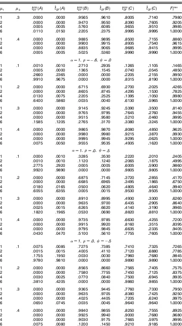
Table 5. Finite Sample Power oftmin

DF(i),OtDF(i) foriDA,B,C, andF

max

T : True DGP is Mixed Model Œ1 Œ3 tminDF(A) OtDF(A) t

min

DF(B) tODF(B) t

min

DF(C) OtDF(C) F

max

T

D11 D001 –D00

1 .1 .0005 .0005 .3070 .3345 02115 01900 02100

2 .0015 .0015 .0760 .0845 01770 01640 04350

4 .2545 .2615 .0000 .0000 06180 06175 09890

6 .9920 .9805 .0000 .0000 09930 09915 100000

1 .2 .0000 .0000 .6450 .6720 03100 02335 03650

2 .0000 .0000 .5835 .6130 02735 01525 06625

4 .0110 .0115 .0380 .0455 05065 04995 09960

6 .5835 .5720 .0000 .0000 09645 09605 100000

1 .3 .0000 .0000 .8705 .8820 04750 03325 06075

2 .0000 .0000 .9480 .9545 05885 02540 08525

4 .0005 .0005 .4920 .5290 04235 03610 09995

6 .1360 .1350 .0250 .0320 09245 09190 100000

1 .4 .0000 .0000 .9740 .9770 06530 03930 08595

2 .0000 .0000 .9950 .9970 08010 02950 09660

4 .0005 .0000 .9600 .9695 05945 02545 09985

6 .0330 .0350 .3915 .4430 08350 08285 100000

D11 D061 –D00

1 .1 .1025 .1110 .7845 .7945 07480 07295 07015

2 .0635 .0690 .4970 .5185 08035 07875 08150

4 .3505 .3610 .0825 .0890 09720 09630 09905

6 .9905 .9905 .0040 .0045 100000 100000 100000

1 .2 .0000 .0000 .8875 .9015 07695 07240 07375

2 .0005 .0010 .7855 .8040 08000 07645 08625

4 .0025 .0030 .2525 .2775 09650 09585 09960

6 .3135 .3505 .0500 .0590 09985 09985 100000

(continued)

Table 5 (continued)

Œ1 Œ3 tDFmin(A) OtDF(A) t

min

DF(B) OtDF(B) t

min

DF(C) OtDF(C) F

max

T

1 .3 .0000 .0000 .9565 .9610 08005 07140 07980

2 .0000 .0000 .9470 .9550 08390 07605 09205

4 .0005 .0005 .5760 .6085 09655 09510 09985

6 .0110 .0150 .2205 .2375 09995 09995 100000

1 .4 .0000 .0000 .9885 .9895 08500 07155 08860

2 .0000 .0000 .9900 .9915 08935 07540 09615

4 .0000 .0000 .8835 .9065 09685 09415 09995

6 .0005 .0005 .5025 .5360 09990 09990 100000

D11 D ƒ061 –D00

1 .1 .0010 .0010 .2710 .2935 01265 01105 01465

2 .0005 .0000 .1365 .1545 00740 00545 04850

4 .2660 .2365 .0000 .0000 02205 02155 09950

6 .9910 .9675 .0000 .0000 08315 08190 100000

1 .2 .0000 .0000 .6715 .6930 02700 02025 04265

2 .0000 .0000 .8605 .8745 04295 01530 07825

4 .0130 .0075 .2205 .2525 01395 01050 09980

6 .6400 .5860 .0035 .0040 06130 05965 100000

1 .3 .0000 .0000 .9145 .9245 05390 03500 08140

2 .0000 .0000 .9765 .9795 07645 02760 09455

4 .0000 .0000 .9515 .9580 05210 00460 09995

6 .1585 .1205 .2765 .3170 03380 03245 100000

1 .4 .0000 .0000 .9865 .9870 08080 04850 09625

2 .0000 .0000 .9980 .9980 09215 03870 09930

4 .0000 .0000 .9995 .9945 09295 00625 100000

6 .0075 .0050 .9555 .9535 04935 01620 100000

D11 D001 –D05

1 .1 .0000 .0010 .3285 .3530 02220 02010 02405

2 .0010 .0010 .1120 .1240 02065 01875 04995

4 .2775 .2920 .0005 .0005 06005 05900 09860

6 .9920 .9890 .0000 .0000 09805 09805 100000

1 .2 .0000 .0000 .6875 .7145 03720 02855 04170

2 .0000 .0000 .6685 .6965 03495 01865 06750

4 .0180 .0165 .0500 .0620 04805 04640 09940

6 .6055 .6355 .0005 .0015 09530 09505 100000

1 .3 .0000 .0000 .8910 .8995 04930 03300 06260

2 .0000 .0000 .9635 .9700 06435 02905 08640

4 .0025 .0015 .6265 .6620 04140 03190 09965

6 .1820 .1965 .0530 .0690 08820 08810 100000

1 .4 .0000 .0000 .9735 .9785 06630 04255 07200

2 .0000 .0000 .9915 .9920 08160 03515 08395

4 .0000 .0000 .9795 .9845 06635 02335 09405

6 .0430 .0470 .5100 .5610 07755 07605 100000

D11 D001 –D ƒ05

1 .1 .0075 .0085 .7275 .7385 07410 07325 07265

2 .0015 .0015 .4005 .4110 07120 06880 07785

4 .1755 .1950 .0030 .0030 07960 07680 09845

6 .9780 .9810 .0000 .0000 09890 09890 100000

1 .2 .0000 .0000 .8565 .8660 07565 07405 07575

2 .0000 .0000 .7580 .7755 07450 07125 08375

4 .0030 .0025 .0770 .0840 07500 06945 09935

6 .3810 .4205 .0000 .0000 09860 09855 100000

1 .3 .0000 .0000 .9365 .9445 07760 07330 07950

2 .0000 .0000 .9635 .9705 08380 07425 09250

4 .0000 .0000 .4025 .4405 07205 06240 09975

6 .0650 .0745 .0035 .0045 09640 09640 100000

1 .4 .0000 .0000 .9840 .9855 08250 07555 08925

2 .0000 .0000 .9925 .9940 09000 07680 09680

4 .0000 .0000 .9030 .9175 07665 05975 09995

6 .0075 .0080 .1200 .1450 09210 09185 100000

NOTE: 5% nominal size, mixed model DGP:y_tD(C)y_tƒ1ƒytƒ2C(1C–L)[Œ1DUctCŒ3DTtcCet].

the power of the crash model statistics decreases withŒ3 and

the power of the changing growth statistics increases withŒ3.

Therefore,tmin

DF4A5 and OtDF4A5 [tminDF4B5 andtODF4B5] can fail

to reject the unit-root null if the true data-generating process is given by the mixed model with a relatively largeŒ3 (Œ1).

5. When the break occurs according to mixed model, the behavior of tmin

DF4C5 and OtDF4C5 is sometimes erratic in that

their power does not always increase with the size ofŒ1 and

Œ3, except when 41 –5D401 065. The power of t min

DF4C5 and O

tDF4C5 tends to fall slightly with the size of Œ3 when Œ1 is

large. The behavior oftmin

DF4C5andOtDF4C5is even more erratic

when Œ3 is Žxed and Œ1 increases. On the other hand,F max

T

has the desirable property in that its power always increases with the size ofŒ1 andŒ3.

6. In all cases, the power ofFmax

T is greater than the power

oftmin

DF4C5andOtDF4C5except when the magnitude of intercept

break or slope break is relatively small. In these cases, the use ofFmax

T does not result in large loss of power.

Given that the power ofFmax

T is larger than the mixed-model

statistics [tmin

DF4C5 and OtDF4C5], it would to be interesting to

ascertain how much of the power ofFmax

T can be attributed to

the break in the trend, that is,Œ16D0 orŒ36D0 or both. The

size of all statistics under the unit-root null hypothesis when there is a break in the intercept and/or slope was calculated. The results, available on request, indicate that the size of all statistics is close to the nominal size when the break mag-nitudes are small. However, the size of Fmax

T increases with

the break magnitudes. In all cases, the size ofFmax

T is slightly

larger than the size oftmin

DF4C5andtODF4C5, and this difference

in size increases slightly with the break magnitudes.

Simulation evidence presented by Vogelsang and Perron (1998) illustrated that all statistics considered within the IO model framework retain their size and power properties if the break in the trend function occurs according to the AO model. While the break in the trend is abrupt and instantaneous within the AO framework, the break in the trend is more gradual within the IO framework. In unreported simulations, we cal-culated the Žnite sample size and power of all IO statistics when the break occurs according to the AO model. Our results indicate that, in general, the size and power properties of all statistics remain the same whether the break occurs according to the AO model or the IO model. However, in most cases, the power oftmin

DF4C5,tODF4C5, andFTmax is larger when the break

occurs according to the AO model compared to their power when the break occurs according to the IO model. The only exception occurs in the changing growth model simulation, where the power ofOtDF4C5levels off with an increase in the

size of the slope break. The AO model simulation results are available from the author on request.

4. EMPIRICAL RESULTS FOR NELSON

AND PLOSSER DATA

In this section, we revaluate the evidence regarding the pres-ence of a unit-root in all Nelson and Plosser (1982) series, except unemployment, and postwar U.S. quarterly real GNP. The natural logarithms of all series were analyzed, except for the interest rate series, which was analyzed in level form.

Empirical evidence for the Nelson–Plosser data can be found in Zivot and Andrews (1992), Perron (1997), Nunes et al. (1997), Murray and Zivot (1998), and Murray and Nelson (2000). Although these studies do not prespecify the location of break, they retain Perron’s (1989) characterization of the form of break under the alternative hypothesis. In particular, Perron (1989) speciŽed the changing growth model for quar-terly real GNP, the mixed model for real wages and common stock prices, and the crash model for all remaining series. However, Perron’s (1989) speciŽcation of the form of break is based on his selection of the great crash of 1929 for all Nelson–Plosser series and the oil price shock of 1973 for quar-terly real GNP series as appropriate break-dates. We argue that once the location of break is treated as unknown, the form of break should also be treated as unknown. Therefore, one must proceed with the most general characterization of the break under the alternative hypothesis, namely, a simultaneous break in the intercept and slope.

Empirical evidence for all Nelson and Plosser (1982) series and quarterly real GNP when the mixed model is used as the appropriate alternative is presented. The k4t-sig5 method of Perron and Vogelsang (1992) is used to determine the appro-priate order of the lag-truncation parameter in regression (10). Following Zivot and Andrews (1992),k-maxD8 is used for the Nelson–Plosser (1982) series and k-maxD12 for quar-terly real GNP. Table 6 reports the calculated statisticstmin

DF4C5, O

tDF4C5, andFTmax for each series, and the corresponding

esti-mated break-dates which are denoted byTb_b4tmin

DF51bTb4OtDF5, and

b

T_b4Fmax

T 5, respectively. The results for regression (10)

corre-sponding to the different estimated break-dates are presented in Table 7. [The results for common stock prices and real wages given in table 6 of Zivot and Andrews (1992) were found to be incorrect. The estimated regression results for real wages with T_bD1940 and kD8 yield the results reported by Zivot and Andrews (1992), but thetstatistic on the ãy_tƒ8

was found to be 1.2277, which is less than 1.6. Although the estimated regression results for common stock prices with T_bD1936 and kD1 yield the results reported by Zivot and Andrews (1992), it was found that with kD3 the tstatistic onãytƒ3is 1.96, which is greater than 1.6. Therefore, in both

cases the k4t-sig5 procedure for choosing the lag-truncation parameter was not applied correctly.]

First, consider the results for tmin

DF4C5 and bTb4tDFmin5. If the

asymptotic critical values are used fortmin

DF4C5given by Zivot

and Andrews (1992), the unit-root null is rejected at the 1% signiŽcance level for real GNP, nominal GNP, and indus-trial production; at the 2.5% signiŽcance level for real per capita GNP, common stock prices, and real wages; at the 5% signiŽcance level for employment, nominal wages, and quar-terly real GNP; and at the 10% signiŽcance level for money stock. The unit-root null for the GNP deator, consumer prices, velocity, and interest rate series were not rejected. Of the series for which the unit-root null is rejected, the esti-mated break-date Tbb4tDFmin5 does not coincide with the great

crash (1929) for real per capita GNP, money stock, common stock prices, and real wages. In addition, the estimated break-date for quarterly real GNP does not coincide with the oil price shock of 1973. The evidence against the unit-root null

Table 6. Empirical Results for the Nelson–Plosser (1982) Data and Quarterly Real GNP

Series tmin

DF(C) bTb(tDFmin) tODF(C) bTb(OtDF) FTmax Tb(FTmax)

Real GNP ƒ506577

(a1c) _{1929 ƒ5}

06577

(b1b) _{1929 10}

09804

(b1c) ₁₉₂₉ Nominal GNP ƒ601741(

a1b) _{1929 ƒ6}

01741(

a1a) _{1929 13}

00122(

a1b) ₁₉₂₉

Real per capita GNP ƒ502983

(b1d) _{1938 ƒ5}

02983

(c1c) _{1938 10}

02524

(b1d) ₁₉₃₈ Industrial production ƒ508192

(a1c) _{1929 ƒ5}

08192

(a1b) _{1929 12}

00478

(a1b) ₁₉₂₉ Employment ƒ501995

(c10)

1929 ƒ501995

(c1d) _{1929 10}

02154

(c1d) ₁₉₂₉

GNP de‘ator ƒ401723 1929 ƒ401723 1920 805103 1920

Consumer prices ƒ305120 1893 ƒ201086 1869 803915 1863

Nominal wages ƒ502147( c10)

1929 ƒ306338 1920 909920(

c1d) ₁₉₂₀

Money stock ƒ409709

(d10)

1930 ƒ409709

(d1d) _{1930 8}

07065 1930

Velocity ƒ309737 1929 ƒ309737 1929 505704 1929

Interest rate ƒ108785 1963 ƒ103131 1964 908964(

c1d) ₁₉₆₄

Common stock prices ƒ505152

(b1d) _{1939 ƒ5}

05015

(b1c) _{1936 10}

02942

(b1d) ₁₉₃₉ Real wages ƒ504509

(b1d) _{1940 ƒ5}

04509

(b1c) _{1940 11}

03206

(a1c) ₁₉₄₀ Quarterly real GNP ƒ501135

(c10)

1964.IV ƒ501135

(d1d) _{1964.IV 8}

07649 1964.IV

NOTE: Mixed-model regression:y_tD OŒ0C OŒ1DUt(Tb)C OŒ2tC OŒ3DTt(Tb)C Oytƒ1CPk

ü

jD1cOjãytƒjC Oet. The small letters in parentheses

that appear as superscript indicate the signi’cance of these statistics. The ’rst letter in the parentheses indicates signi’cance with respect to the asymptotic critical values, and the second letter indicates signi’cance with respect to the appropriate ’nite sample critical values. a, b, c, and d indicate signi’cance at the 1%, 2.5%, 5%, and 10% signi’cance level, and . appears if the statistic is not signi’cant at the 10% signi’cance level. The asymptotic and ’nite sample critical values oftmin

DF(C)are taken from table 4 in Zivot and

Andrews (1992) and table 1 in Perron (1997), respectively. The asymptotic and ’nite sample critical values forOtDF(C)were obtained

from table 3 in Vogelsang and Perron (1998). The asymptotic and ’nite sample critical values forF_Tmaxwere taken from Table 1 in this article.‹0D005 was used.

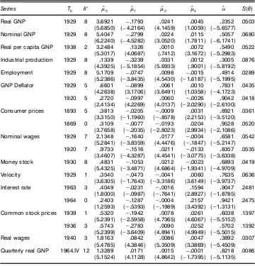
Table 7. Estimated Regressions for the Nelson–Plosser (1982) Data and Quarterly Real GNP

Series Tb k

ü _ŒO

0 ŒO1 ŒO2 ŒO3 O S(eO)

Real GNP 1929 8 306921 ƒ01793 00241 00045 02352 .0503

(506850) (ƒ402164) (401459) (100059) (ƒ506577)

Nominal GNP 1929 8 504047 ƒ02799 00224 00115 05057 .0680

(602240) (ƒ405282) (300520) (107811) (ƒ601741)

Real per capita GNP 1938 2 302484 01326 00010 00072 05490 .0522

(503017) (400687) (07412) (301672) (ƒ502983)

Industrial production 1929 8 01339 ƒ03239 00331 00012 03005 .0876

(403925) (ƒ501854) (506933) (09001) (ƒ508192)

Employment 1929 8 501709 ƒ00747 00098 ƒ00015 04914 .0289

(502386) (ƒ308435) (405430) (ƒ106187) (ƒ501995)

GNP De‘ator 1929 5 06601 ƒ00899 00061 00010 07831 .0435

(402638) (301706) (306491) (100358) (ƒ401723)

1920 5 02720 ƒ00997 00060 ƒ00026 09042 .0418

(204134) (402269) (400137) (ƒ200290) (ƒ206100)

Consumer prices 1893 5 03813 ƒ00205 ƒ00009 00031 08921 .0361

(303150) (ƒ101960) (ƒ08578) (202153) (ƒ305120)

1869 0 03109 ƒ00077 ƒ00193 00204 09528 .0520

(307658) (ƒ02035) (ƒ208023) (209934) (ƒ201086)

Nominal wages 1929 7 201348 ƒ01640 00177 ƒ00004 06581 .0542

(502841) (ƒ308359) (404476) (ƒ01847) (ƒ502147)

1920 7 09733 ƒ01516 00211 ƒ00133 08357 .0535

(304607) (ƒ403287) (404541) (ƒ300775) (ƒ306338)

Money stock 1930 8 04831 ƒ01053 00212 ƒ00023 06893 .0419

(504325) (ƒ304871) (406864) (ƒ109341) (ƒ409709)

Velocity 1929 1 03540 ƒ00473 ƒ00041 00060 07635 .0636

(306305) (ƒ107643) (ƒ303186) (306149) (ƒ309737)

Interest rate 1963 3 04049 ƒ00231 ƒ00016 01594 09047 .2481

(108000) (ƒ00987) (ƒ07641) (208927) (ƒ108785)

1964 0 02403 ƒ01287 ƒ00004 02157 09421 .2475

(102593) (ƒ05393) (ƒ01989) (304392) (ƒ103131)

Common stock prices 1939 1 05320 ƒ01942 00078 00261 06038 .1397

(502391) (ƒ205958) (407365) (406067) (ƒ505152)

1936 3 05743 ƒ02783 00090 00252 05702 .1392

(502399) (ƒ306409) (408941) (409949) (ƒ505015)

Real wages 1940 3 108163 00842 00086 00047 03892 .0307

(504785) (403846) (503509) (303869) (ƒ504509)

Quarterly real GNP 1964.IV 12 103289 00171 00015 ƒ00001 08218 .0086

(501524) (401128) (408642) (ƒ107395) (ƒ501135)

NOTE: Mixed-model regression:y_tD OŒ0C OŒ1DUt(Tb)C OŒ2tC OŒ3DTt(Tb)C Oytƒ1CPk

ü

jD1OcjãytƒjC Oet.Tbis the chosen break-date, küis the value of the lag-truncation parameter chosen according to thek(t-sig) procedure of Perron and Vogelsang (1992) withk -maxD8 for all series except quarterly real GNP, for whichk-maxD12. Thetstatistics appear in parentheses. Thetstatistic forOtests the hypothesis thatD1.S(eO)is the estimated standard deviation of the regression error.

is weakened if the Žnite sample critical values given by Per-ron (1997) are used fortmin

DF4C5with lag-truncation parameter

selected using thek4t-sig5method. With the Žnite sample crit-ical values, the unit-root null for employment, nominal wages, money stock, and quarterly real GNP cannot be rejected.

Because a break is not allowed under the unit-root null hypothesis, these results should be compared to the results of Zivot and Andrews (1992). The unit-root null hypothe-sis is rejected here for money stock, real wages, and quar-terly real GNP in addition to all series for which Zivot and Andrews (1992) rejected the unit-root null. Further, the present evidence is stronger for real per capita GNP. Unlike that of Zivot and Andrews (1992), the break-date estimated here for real per capita GNP is 1938, for money stock is 1930, for common stock prices is 1939, and for quarterly real GNP is 1964, fourth quarter. The estimated break-date coincides with the great crash of 1929 for real GNP, nominal GNP, indus-trial production, employment, and nominal wages. In cases for which the unit-root null is rejected, one would like to deter-mine the signiŽcance of the trend function coefŽcients Œ0,

Œ1, Œ2, andŒ3 evaluated atTbb4tminDF5. Given that the location

of break is estimated byTb_b4tmin

DF5, the asymptotic distribution

of t statistics for H02 ŒiD0, denoted by tŒOi, (iD0111213)

may not be well approximated by the standard normal distri-bution. In unreported simulations, the empirical distribution of tŒOi (iD0111213) corresponding to the estimated regression at

b

Tb4tDFmin5 was examined. The results indicate that the

empiri-cal distributions oftŒOi (iD01213) are symmetric, have mean

close to zero, but have a slightly larger variance compared to the standard normal distribution. On the other hand, the empir-ical distribution oftŒO1 is bimodal with a much larger variance

compared to the standard normal distribution. [It was found that the empirical distributions oftŒOi (foriD0111213)

evalu-ated atTbb4OtDF5andTbb4FTmax5exhibit similar behavior.] Results

pertaining to the empirical distribution oftŒOi (iD0111213) are

available on request. As a Žrst approximation, the signiŽcance of the intercept coefŽcient (Œ0), the trend coefŽcient (Œ2), and

the slope break coefŽcient (Œ₃) using the critical values from a standard normal distribution are assessed. [However, the sig-niŽcance of the intercept break coefŽcient (Œ1) using the

stan-dard normal critical values is not determined.] The estimated coefŽcients and their respective t statistics are presented in Table 7. It was found that tŒO0 andtŒO2 are signiŽcant for all

series, with the sole exception ofŒ₂ for real per capita GNP, andtŒO3 is signiŽcant for nominal GNP, real per capita GNP,

money stock, common stock prices, real wages, and quarterly real GNP.

Second, the results for tODF4C5 are qualitatively similar to

those ofOtmin

DF4C5. The critical values forOtDF4C5, both

asymp-totic and Žnite sample with lag-truncation parameter chosen according to thek4t-sig5method, can be found in Vogelsang and Perron (1998). Based on the asymptotic critical values, the unit-root null is rejected at the 1% signiŽcance level for nom-inal GNP and industrial production; at the 2.5% signiŽcance level for real GNP, common stock prices, and real wages; at the 5% signiŽcance level for real per capita GNP and employ-ment; and at the 10% signiŽcance level for money stock and quarterly real GNP. The unit-root null cannot be rejected for GNP deator, consumer prices, nominal wages, velocity, and

interest rate. The results for all series are in agreement with the results corresponding to tmin

DF4C5, with the exception of

nominal wages. The estimated break-dateTbb4OtDF5is the same

as Tbb4tDFmin5 for all series for which the unit-root is rejected,

except common stock prices, for which the estimated break-date is 1936. The use of Žnite sample critical values weakens the evidence against the unit-root null somewhat.

Finally, consider the results with Fmax

T . The critical values

forFmax

T , both asymptotic and Žnite sample, are obtained from

Table 1. Based on the asymptotic critical values, the joint null hypothesis can be rejected at the 1% signiŽcance level for nominal GNP, industrial production, and real wages; at the 2.5% level for real GNP, real per capita GNP, and common stock prices; and at the 5% signiŽcance level for employment, nominal wages, and interest rate. The use of Žnite sample critical values leads to a rejection of the joint null hypoth-esis for these series at higher signiŽcance levels. Although Fmax

T fails to rejectH J

0 for the money stock and quarterly real

GNP series, it is borderline signiŽcant at the 10% signiŽcance level. Also,Fmax

T is signiŽcant for the interest rate series. The

estimated break-datebTb4FTmax5 is the same asTbb4tminDF5 for all

series for which the joint null hypothesis is rejected, except for nominal wages and interest rate. The break-date,Tb_b4Fmax

T 5,

for nominal wages is 1920 and is 1964 for interest rate. The failure oftmin

DF4C5andtODF4C5to rejectH02 D1 for the

inter-est rate series, and the signiŽcance ofFmax

T can be explained

as follows. It is reasonable to rule out a nonzero trend (Œ26D0

andŒ36D0) in the presence of a unit-root; see Perron (1988,

p. 304). Therefore, Fmax

T will be signiŽcant either if ——<1

or ifD1 andŒ16D0. Because Vogelsang and Perron (1998)

showed that the limiting distribution oftmin

DF4C5is invariant to

a shift in the intercept under the null, the rejection ofHJ

0 can

be attributed to the presence of a break under the unit-root null hypothesis.

To sum up, our results indicate that the unit-root null hypothesis can be rejected for all series except GNP dea-tor, consumer prices, velocity, and interest rate. Because the form of break was not imposed under the alternative hypoth-esis, the results are robust to possible misspeciŽcation and reveal important information regarding the location and form of break. Consider, for example, the results with real per capita GNP. In this case, the evidence against a unit-root is strength-ened by using the mixed model as the appropriate alternative, and it is found that unlike previous empirical evidence the estimated break-date does not coincide with the great crash but rather the break occurs considerably later in 1938. Also, evidence was uncovered against the unit-root null for money stock and quarterly real GNP when the mixed model is used. The estimated break-date for money stock is 1930, and that for quarterly real GNP is 1964, fourth quarter. The estimated break-date of 1964 for the quarterly real GNP series coincides with the tax cut mentioned by Christiano (1992). In contrast to earlier studies, these results indicate that a slope break coef-Žcient should be included for nominal GNP, real per capita GNP, money stock, and quarterly real GNP.

5. CONCLUSION

In this article, we argued that the practitioner should treat the form of break as unknown when testing for the pres-ence of a unit-root. Earlier studies considered three different