Full Terms & Conditions of access and use can be found at
http://www.tandfonline.com/action/journalInformation?journalCode=ubes20
Download by: [Universitas Maritim Raja Ali Haji] Date: 11 January 2016, At: 22:36
Journal of Business & Economic Statistics
ISSN: 0735-0015 (Print) 1537-2707 (Online) Journal homepage: http://www.tandfonline.com/loi/ubes20
Regime-Specific Predictability in Predictive
Regressions
Jesús Gonzalo & Jean-Yves Pitarakis
To cite this article: Jesús Gonzalo & Jean-Yves Pitarakis (2012) Regime-Specific Predictability in Predictive Regressions, Journal of Business & Economic Statistics, 30:2, 229-241, DOI: 10.1080/07350015.2011.652053
To link to this article: http://dx.doi.org/10.1080/07350015.2011.652053
View supplementary material
Accepted author version posted online: 27 Dec 2011.
Submit your article to this journal
Article views: 348
Supplementary materials for this article are available online. Please go tohttp://tandfonline.com/r/JBES
Regime-Specific Predictability in Predictive
Regressions
Jes ´us G
ONZALODepartment of Economics, Universidad Carlos III de Madrid, Getafe (Madrid) 28903, Spain ([email protected])
Jean-Yves P
ITARAKISEconomics Division, School of Social Sciences, University of Southampton, Southampton SO17 1BJ, UK ([email protected])
Predictive regressions are linear specifications linking a noisy variable such as stock returns to past values of a very persistent regressor with the aim of assessing the presence of predictability. Key complications that arise are the potential presence of endogeneity and the poor adequacy of asymptotic approximations. In this article, we develop tests for uncovering the presence of predictability in such models when the strength or direction of predictability may alternate across different economically meaningful episodes. An empirical application reconsiders the dividend yield-based return predictability and documents a strong predictability that is countercyclical, occurring solely during bad economic times. This article has online supplementary materials.
KEY WORDS: Endogeneity; Persistence; Return predictability; Threshold models.
1. INTRODUCTION
Predictive regressions with a persistent regressor (e.g., divi-dend yields, interest rates, realized volatility) aim to uncover the ability of a slowly moving variable to predict future values of an-other typically noisier variable (e.g., stock returns, GDP growth) within a bivariate regression framework. Their pervasive nature in many areas of economics and finance and their importance in the empirical assessment of theoretical predictions of economic models made this particular modeling environment an important and active area of theoretical and applied research (for instance, see Jansson and Moreira2006and references therein).
A common assumption underlying old and new developments in this area involves working within a model in which the per-sistent regressor enters the predictive regression linearly, thus not allowing for the possibility that the strength and direction of predictability may themselves be a function of some economic factor or time itself. Given this restriction, existing work has fo-cused on improving the quality of estimators and inferences in this environment, characterized by persistence and endogeneity, among other econometric complications. These complications manifest themselves in the form of nonstandard asymptotics, distributions that are not free of nuisance parameters, poor finite-sample approximations, etc. Important recent method-ological breakthroughs have been obtained by Jansson and Moreira (2006), Campbell and Yogo (2006), Valkanov (2003), and Lewellen (2004), while recent applications in the area of financial economics and asset pricing can be found in Cochrane (2008), Lettau and Nieuwerburgh (2008), Bandi and Perron (2008), among others.
The purpose of this article is to instead develop an economet-ric toolkit for uncovering the presence of predictability within regression models with highly persistent regressors when the strength or direction of predictability, if present, may alternate across different economically meaningful episodes (e.g.,
peri-ods of rapid versus slow growth, periperi-ods of high versus low stock market valuation, periods of high versus low consumer confidence, etc.). For this purpose, we propose to expand the traditional linear predictive regression framework to a more gen-eral environment that allows for the possibility that the strength of predictability may itself be affected by observable economic factors. We have in mind scenarios whereby the predictability induced by some economic variable kicks in under particu-lar instances, such as when the magnitude of the variable in question (or some other variable) crosses a threshold but is use-less in terms of predictive power otherwise. Alternatively, the predictive impact of a variable may alternate in sign/strength across different regimes. Ignoring such phenomena by proceed-ing within a linear framework, as has been done in the litera-ture, may mask the forecasting ability of a particular variable and, more generally, mask the presence of interesting and eco-nomically meaningful dynamics. We subsequently apply our methodology to the prediction of stock returns with dividend yields (DY). Contrary to what has been documented in the lin-ear predictability literature, our findings strongly point toward the presence of regimes in which DY-based predictability kicks in solely during bad economic times. More importantly, our analysis also illustrates the fact that the presence of regimes may make predictability appear as nonexistent when assessed within a linear model.
The plan of the article is as follows. Section 2 introduces our model and hypotheses of interest. Section 3 develops the limiting distribution theory of our test statistics. Section 4 explores the finite-sample properties of the inferences devel-oped in Section 3, Section 5 proposes an application, and
© 2012American Statistical Association Journal of Business & Economic Statistics April 2012, Vol. 30, No. 2 DOI:10.1080/07350015.2011.652053
229
Section 6 concludes. All proofs are relegated to the Ap-pendix. Due to space considerations, additional Monte Carlo simulations and further details on some of the proofs are pro-vided as an online supplementary appendix.
2. THE MODEL AND HYPOTHESES
We will initially be interested in developing the limiting dis-tribution theory for a Wald-type test statistic designed to test the null hypothesis of a linear relationship betweenyt+1andxt
against the following threshold alternative
yt+1 =
α1+β1xt+ut+1 qt ≤γ
α2+β2xt+ut+1 qt > γ , (1)
wherextis parameterized as the nearly nonstationary process
xt =ρTxt−1+vt, ρT =1−
c
T, (2)
withc >0, qt=µq+uqt, and ut,uqt, andvt are stationary
random disturbances. The above parameterization allowsxt to
display local to unit root behavior and has become the norm for modeling highly persistent series for which a pure unit root assumption may not always be sensible. The threshold variable
qtis taken to be a stationary process, andγrefers to the unknown
threshold parameter. Underα1=α2andβ1=β2, our model in (1)–(2) coincides with that in Jansson and Moreira (2006) or Campbell and Yogo (2006) and is commonly referred to as a predictive regression model, while underα1=α2, β1=β2=0, we have a constant mean specification.
The motivation underlying our specification in (1)–(2) is its ability to capture phenomena such as regime-specific pre-dictability within a simple and intuitive framework. We have in mind scenarios whereby the slope corresponding to the predictor variable becomes significant solely in one regime. Alternatively, the strength of predictability may differ depending on the regime determined by the magnitude ofqt. The predictive instability in
stock returns that has been extensively documented in the re-cent literature and the vanishing impact of DYs from the 1990s onward in particular (see Ang and Bekaert 2007and also Ta-ble 7) may well be the consequence of the presence of regimes for instance. Among the important advantages of a threshold-based parameterization are the rich set of dynamics it allows us to capture despite its mathematical simplicity, its estimabil-ity via a simple least squares-based approach, and the observ-ability of the variable triggering regime switches, which may help attach a “cause” to the underlying predictability. Following Petruccelli (1992), it is also useful to recall that the piecewise linear structure can be viewed as an approximation to a much wider family of nonlinear functional forms. In this sense, al-though we do not argue that our chosen threshold specification mimics reality, we believe that it offers a realistic approximation to a wide range of more complicated functional forms and to regime-specific behavior in particular. It is also interesting to highlight the consequences that a behavior such as (1)–(2) may have if ignored and if predictability is assessed within a linear specification instead, sayyt=βxt−1+ut. Imposing zero
inter-cepts for simplicity and assuming (1)–(2) holds with someγ0, it is easy to establish that ˆβ →p β1+(β2−β1)P(qt > γ0). This raises the possibility that ˆβ may converge to a quantity that is
very close to zero (e.g., whenP(qt > γ0)≈β1/(β1−β2)) so that tests conducted within a linear specification may frequently and wrongly suggest the absence of any predictability.
Our choice of modelingxtas a nearly integrated process
fol-lows the same motivation as in the linear predictive regression literature, where such a choice for xt has been advocated as
an alternative to proceeding with conventional Gaussian critical values that typically provide poor finite-sample approximations to the distribution oftstatistics. In the context of a stationary AR(1) for instance, Chan (1988) demonstrated that for values ofT(1−ρ)≥50, the normal distribution offers a good approx-imation, while forT(1−ρ)≤50, the limit obtained assuming near integratedness works better when the objective involves conducting inferences about the slope parameter of the AR(1) (see also Cavanagh, Elliott, and Stock1995for similar points in the context of a predictive regression model). Models that combine persistent variables with nonlinear dynamics as (1)– (2) offer an interesting framework for capturing stylized facts observed in economic data. Within a univariate setting (e.g., threshold unit root models), recent contributions toward their theoretical properties have been obtained by Caner and Hansen (2001) and Pitarakis (2008).
In what follows, the threshold parameterγ is assumed un-known, with γ ∈Ŵ=[γ1, γ2], and γ1 and γ2 are selected such thatP(qt ≤γ1)=π1>0 andP(qt ≤γ2)=π2<1, as in Caner and Hansen (2001). We also defineI1t ≡I(qt ≤γ) and
I2t ≡I(qt > γ) but replace the threshold variable with a
uni-formly distributed random variable, making use of the equality
I(qt ≤γ)=I(F(qt)≤F(γ))≡I(Ut ≤λ). Here, F(.) is the
marginal distribution of qt, and Ut denotes a uniformly
dis-tributed random variable on [0,1]. Before proceeding further, it is also useful to reformulate (1) in matrix format. Letting
ydenote the vector stacking yt+1 andXi the matrix stacking
(Iit xtIit) fori=1,2, we can write (1) asy =X1θ1+X2θ2+u or y =Zθ+u, with Z=(X1 X2), θ=(θ1, θ2), and θi =
(αi, βi)′ i=1,2. For later use, we also define X=X1+X2 as the regressor matrix that stacks the constant andxt. It is now
easy to see that for givenγorλ, the homoscedastic Wald statis-tic for testing a general restriction onθ, sayRθ=0, is given by
WT(λ)=θˆ′R′(R(Z′Z)−1R′)−1Rθ /ˆ σˆu2, with ˆθ=(Z′Z)−
1Z′y,
and ˆσu2=(y′y−2i=1y′Xi(X′iXi)−1X′iy)/T is the residual
variance obtained from (1). In practice, since the threshold pa-rameter is unidentified under the null hypothesis, inferences are conducted using the SupWald formulation, expressed as supλ∈[π1,π2]WT(λ), withπ1 =F(γ1) andπ2=F(γ2).
Through-out this article, the practical implementation of our SupWald statistics will use 10% trimming at each end of the sample.
In the context of our specification in (1)–(2), we will initially be interested in the null hypothesis of linearity given byHA
0 :
α1=α2, β1=β2. We write the corresponding restriction matrix asRA=[I −I], withI denoting a 2×2 identity matrix and
the SupWald statistic supλWTA(λ). At this stage, it is important
to note that the null hypothesis given by H0A corresponds to the linear specification yt+1=α+βxt+ut+1 and thus does not test predictability per se sincext may appear as a predictor
under both the null and the alternative hypothesis. Thus, we also consider the null given byH0B :α1=α2, β1=β2=0, with the corresponding SupWald statistic written as supλWTB(λ), where
nowRB =[1 0 −1 0,0 1 0 0,0 0 0 1]. Under this null
hypothesis, the model is given byyt+1=α+ut+1and the test is expected to have power against departures from both linearity and predictability.
3. LARGE-SAMPLE INFERENCE
Our objective here is to investigate the asymptotic proper-ties of Wald-type tests for detecting the presence of thresh-old effects in our predictive regression setup. We initially obtain the limiting distribution of WA
T(λ) under the null
hy-pothesisHA
0 :α1=α2, β1 =β2. We subsequently turn to the joint null hypothesis of linearity and no predictability given by
H0B :α1=α2, β1=β2=0, and explore the limiting behavior ofWTB(λ).
Our operating assumptions about the core probabilistic struc-ture of (1)–(2) will closely mimic the assumptions imposed in the linear predictive regression literature but will occa-sionally also allow for a greater degree of generality (e.g., Cavanagh et al.1995; Campbell and Yogo2006; Jansson and Moreira2006, among others). Specifically, the innovationsvt
will be assumed to follow a general linear process we write asvt =(L)et, where(L)=
the form of a martingale difference sequence (m.d.s.) with re-spect to an appropriately defined information set. More formally, lettingwt =(ut, et)′ andF
continuous and strictly increasing distributionF(.) and is such thatuqt is a strictly stationary, ergodic, and strong mixing
se-quence, with mixing numbersαmsatisfying
∞
One implication of Assumption 1 and the properties of
(L) is that a functional central limit theorem holds for the joint process wt =(ut, vt)′ (see Phillips 1987).
More formally,[tT r=1]wt/
√
T ⇒B(r)=(Bu(r), Bv(r))′, with
the long-run variance of the bivariate Brownian motion
B(r) being given by =∞k=−∞E[w0w′k]=[(ω
assumption. Given our parameterization ofvt and the m.d.s.
assumption forut, we haveωuv=σue(1) andω2v=σ
sided autocovariance so thatω2
v =σv2+2λvv≡σe2
tion in Assumption 1 imposes a particular structure on. For instance, since serial correlation in ut is ruled out, we have
ω2
u=σu2. It is worth emphasizing, however, that while
rul-ing out serial correlation in ut, our assumptions allow for a
sufficiently general covariance structure linking (1)–(2) and a general dependence structure for the disturbance terms driv-ing xt and qt. The m.d.s. assumption onut is a standard
as-sumption that has been made throughout all recent research
on predictive regression models (for instance, see Campbell and Yogo 2005 and references therein; Jansson and Moreira 2006) and appears to be an intuitive operating framework, given that many applications take yt+1 to be stock returns. Writing
=∞k=1E[wtw′t−k]=[(λuu, λuv),(λvu, λvv)], it is also
use-ful to explicitly highlight the fact that within our probabilistic environment,λuu=0 andλuv=0 due to the m.d.s. property of
theu′
ts, whileλvvandλvumay be nonzero.
Regarding the dynamics of the threshold variableqtand how
it interacts with the remaining variables driving the system, Assumption 1 requiresqt−j’s to be orthogonal toutforj ≥1.
Sinceqtis stationary, this is in a way a standard regression model
assumption and is crucial for the development of our asymptotic theory. We note, however, that our assumptions allow for a broad level of dependence between the threshold variableqt and the
other variables included in the model (e.g.,qt may be
contem-poraneously correlated with both ut andvt). At this stage, it
is perhaps also useful to reiterate the fact that our assumption about the correlation ofqt with the remaining components of
the system is less restrictive than what is typically found in the literature on marked empirical processes or functional coeffi-cient models such asyt+1=f(qt)xt+ut+1, which commonly takeqt to be independent ofutandxt.
Since our assumptions also satisfy Caner and Hansen’s (2001) framework, from their theorem 1, we can write
[T r]
t=1 utI1t−1/ √
T ⇒Bu(r, λ) as T → ∞, with Bu(r, λ)
de-noting a two-parameter Brownian motion with covariance
σu2(r1∧r2)(λ1∧λ2) for (r1, r2),(λ1, λ2)∈[0,1]2 and where
a∧b≡min{a, b}. Noting thatBu(r,1)≡Bu(r), we will also
make use of a particular process, known as a Kiefer process and defined as Gu(r, λ)=Bu(r, λ)−λBu(r,1). A Kiefer process
on [0,1]2 is Gaussian with zero mean and covariance func-tionσ2
sumptions, it follows directly from lemma 3.1 in Phillips (1988) thatx[T r]/
√
T ⇒Kc(r). For notational clarity in what follows,
it is important to recall that Kc(r) and all our other processes
indexed by eitheruorvare univariate.
3.1 TestingHA
0 :α1=α2, β1=β2
Having outlined our key operating assumptions, we now turn to the limiting behavior of our test statistics. We will initially concentrate on the null hypothesis given byH0A:α1=α2, β1=
β2and the behavior of supλWTA(λ), which is summarized in the
following proposition.
Proposition 1. Under the null hypothesis H0A:α1=
α2, β1=β2, Assumptions 1 and 2, and as T → ∞, the lim-iting distribution of the SupWald statistic is given by:
sup
where Kc(r)=(1, Kc(r))′, Gu(r, λ) is a Kiefer process and
Kc(r) an Ornstein-Uhlenbeck process.
Although the limiting random variable in (3) appears to de-pend on unknown parameters, such as the correlation between
Bu andBv,σu2, and the near-integration parameterc, a closer
analysis of the expression suggests instead that it is equivalent to a random variable given by a quadratic form in normalized Brownian bridges, identical to the one that occurs when testing for structural breaks in a purely stationary framework. We can write it as
sup
λ
BB(λ)′BB(λ)
λ(1−λ) , (4) withBB(λ) denoting a standard bivariate Brownian bridge (re-call that a Brownian bridge is a zero mean Gaussian process with covariance λ1∧λ2−λ1λ2). This result follows from the fact that the processesKc(r) andGu(r, λ) appearing in the
stochas-tic integrals in (3) are uncorrelated and thus independent since Gaussian. Indeed, as in (3), gives the Brownian bridge process in (4), which is also the unconditional distribution since it is not depen-dent on a realization of Kc(r) (see also lemma 5.1 in Park
and Phillips 1988). Obviously, the discussion trivially car-ries through to Kc and Gu since E[Kc(r2)Gu(r1, λ1)]′=
E[Gu(r1, λ1) Kc(r2)Gu(r1, λ1)]′=[0 0]′.
The result in Proposition 1 is unusual and interesting for a variety of reasons. It highlights an environment in which the null distribution of the SupWald statistic no longer depends on any nuisance parameters as it is typically the case in a purely station-ary environment and thus no bootstrapping schemes are needed for conducting inferences. In fact, the distribution presented in Proposition 1 is extensively tabulated in Andrews (1993), and Hansen (1997) providedp-value approximations that can be used for inference purposes. More recently, Estrella (2003)
also provided exactp-values for the same distribution. Finally and perhaps more importantly, the limiting distribution does not depend onc, the near-integration parameter, which is another unusual feature of our framework.
All these properties are in contrast with what has been doc-umented in the recent literature on testing for threshold effects in purely stationary contexts. In Hansen (1996) for instance, the author investigated the limiting behavior of a SupLM-type test statistic for detecting the presence of threshold nonlin-earities in purely stationary models. There, it was established that the key limiting random variables depend on numerous nuisance parameters involving unknown population moments of variables included in the fitted model. From theorem 1 in Hansen (1996), it is straightforward to establish, for in-stance, that under stationarity, the limiting distribution of a Wald-type test statistic would be given byS∗(λ)′M∗(λ)−1S∗(λ),
withM∗(λ)=M(λ)−M(λ)M(1)−1M(λ), andS∗(λ)=S(λ)−
M(λ)M(1)−1S(1). Here,M(λ)
=E[X′
1X1] andS(λ) is a zero mean Gaussian process with varianceM(λ). Since in this context the limiting distribution depends on the unknown model-specific population moments, the practical implementation of inferences is through a bootstrap-style methodology.
One interesting instance worth pointing out, however, is the fact that this limiting random variable simplifies to a Brown-ian bridge type of limit when the threshold variable is taken as exogenous in the senseM(λ)=λM(1). Although the compar-ison with the present context is not obvious since we takext
to be near-integrated and we allow the innovations inqt to be
correlated with those ofxt, the force behind the analogy comes
from the fact thatxtandqthave variances with different orders
of magnitude. In a purely stationary setup, takingxtas
station-ary and the threshold variable as some uniformly distributed random variable leads to results such asx2
tI(Ut ≤λ)/T
is instrumental in leading to the Brownian bridge type of limit in Hansen’s (1996) framework. If nowxt is taken as a nearly
integrated process and regardless of whether its shocks are corre-lated withUtor not, we havext2I(Ut≤λ)/T2⇒λ
K2
c(r),
which can informally be viewed as analogous to the previous scenario. Heuristically, this result follows by establishing that asymptotically, objects interactingxt/
√
(see also Caner and Hansen2001, p. 1585; Pitarakis2008). This would be similar to arguing that xt/
√
T and I1t are
asymp-totically uncorrelated in the sense that their sample covariance (normalized byT) is zero in the limit.
3.2 TestingHB
0 :α1=α2, β1=β2=0
We next turn to the case where the null hypothesis of interest tests jointly the absence of linearity and no predictive power; that is, we focus on testingHB
0 :α1=α2, β1=β2=0 using the supremum ofWB
T(λ). The following proposition summarizes
its limiting behavior.
Proposition 2. Under the null hypothesis H0B :α1=
α2, β1=β2 =0, Assumptions 1 and 2, and as T → ∞, the
limiting distribution of the SupWald statistic is given by the remaining variables are as in Proposition 1.
Looking at the expression of the limiting random variable in (5), we note that it consists of two components, with the second one being equivalent to the limiting random variable we obtained under Proposition 1. Under endogeneity, the first component on the right-hand side of (5) is more problematic in the sense that it does not simplify further due to the fact thatKc∗(r) andBu(r,1)
are correlated, sinceωuvmay take nonzero values. However, if
we were to rule out endogeneity by settingωuv=0, then it is
interesting to note that the limiting distribution of the SupWald statistic in Proposition 2 takes the following simpler form
sup variate standard normally distributed random variable. The first component on the right-hand side of either (5) or (6) can be rec-ognized as theχ2(1) limiting distribution of the Wald statistic for testingH0:β=0 in the linear specification
yt+1 =α+βxt+ut+1, (7) and the presence of this first component makes the test powerful in detecting deviations from the null (see Rossi 2005 for an illustration of a similar phenomenon in a different context).
Our next concern is to explore ways of making (5) opera-tional since, as it stands, the first component of the limiting random variable depends on model-specific moments and can-not be universally tabulated. For this purpose, it is useful to can-note that the problems arising from the practical implementation of (5) are partly analogous to the difficulties documented in the single-equation cointegration testing literature, where the goal was to obtain nuisance-parameter-free chi-squared asymptotics for Wald-type tests onβ in (7) despite the presence of endo-geneity (see Phillips and Hansen1990; Saikkonen1991,1992). As shown by Elliott (1998), however, inferences about β in (7) can no longer be mixed normal whenxt is a near-unit root
process. It is only very recently that Phillips and Magdalinos (2009) (PM09 thereafter) reconsidered the issue and resolved the difficulties discussed in Elliott (1998) via the introduction of a new instrumental-variable-type estimator ofβin (7). Their method is referred to as IVX estimation since the relevant IV is constructed solely via a transformation of the existing regressor
xt. It is this same method that we propose to adapt to our present
context.
Before proceeding further, it is useful to note thatWB T(λ) can
be expressed as the sum of the following two components:
WTB(λ)≡σˆ the residual variance obtained from the same linear specifica-tion. Although not of direct interest, this reformulation ofWB
T(λ)
can simplify the implementation of the IVX version of the Wald statistic since the setup is now identical to that of PM09 and involves constructing a Wald statistic for testingH0:β =0 in (7); that is, we replace WT(β =0) in (8) with its IVX-based
version, which is shown to be asymptotically distributed as a
χ2(1) random variable that does not depend on the noncentral-ity parametercor other endogeneity-induced parameters. Note that although PM09 operated within a model without an in-tercept, Stamatogiannis (2010) and Kostakis, Magdalinos, and Stamatogiannis (2010) have also established the validity of the theory in models with a fitted constant term.
The IVX methodology starts by choosing an artificial slope coefficient, say
tain an IV estimator of β in (7) and to construct the corre-sponding Wald statistic for testing H0:β=0. Through this judicious choice of the instrument, PM09 showed that it is possible to clean out the effects of endogeneity even within the near-unit root case and to subsequently obtain an estima-tor ofβthat is mixed normal under a suitable choice ofδ(i.e.,
δ∈(2/3,1)) and settingcz=1 (see PM09, pp. 7–12). More
im-portantly, the resulting limiting distribution of the Wald statistic for testingβ =0 in (7) no longer depends on the noncentrality parameterc.
Following PM09 and Stamatogiannis (2010) and lettingy∗
t, Note that contrary to PM09 or Stamatogiannis (2010), we do not need a bias correction term in the numerator of ˜βivxsince we operate under the assumption thatλuv =0. The corresponding
IVX-based Wald statistic for testingH0:β =0 in (7) is now is also asymptotically equivalent to ˆσlin2 since the least squares estimator of β remains consistent. Under the null hypothesis
H0B, we also have that these two residual variances are in turn asymptotically equal to ˆσu2so that ˆσlin2/σˆu2≈1 in (8).
We can now introduce our modified Wald statistic, say
WTB,ivx(λ), for testingHB
0 :α1 =α2, β1=β2=0 in (1) as
WTB,ivx(λ)=WTivx(β=0)+WTA(λ). (12) Its limiting behavior is summarized in the following proposition.
Proposition 3. Under the null hypothesis H0(B):α1=
α2, β1=β2=0, Assumptions 1 and 2, δ∈(2/3,1) in (10), and asT → ∞, we have
sup
λ
WTB,ivx(λ)⇒W(1)2+sup
λ
BB(λ)′BB(λ)
λ(1−λ) , (13) withBB(λ) denoting a standard Brownian bridge.
Our result in (13) highlights the usefulness of the IVX-based estimation methodology since the resulting limiting distribution of the SupWald statistic is now equivalent to the one obtained under strict exogeneity (i.e., underωuv=0) in (6). The practical
implementation of the test is also straightforward, requiring nothing more than the computation of an IV estimator.
4. FINITE-SAMPLE ANALYSIS
4.1 TestingHA
0 :α1=α2, β1=β2
Having established the limiting properties of the SupWald statistic for testingH0A, our next goal is to illustrate the finite-sample adequacy of our asymptotic approximation and empiri-cally illustrate our theoretical findings. It will also be important to highlight the equivalence of the limiting results obtained in Proposition 1 to the Brownian bridge type of limit documented in Andrews (1993) and for which Hansen (1997) obtainedp-value approximations and Estrella (2003), exactp-values. Naturally, this allows us to evaluate the size properties of our tests as well.
Our data-generating process (DGP) underHA
0 is given by the following set of equations:
yt =α+βxt−1+ut,
xt =
1−Tc
xt−1+vt,
vt =ρvt−1+et, (14)
withutandetboth NID(0,1), while the fitted model is given by
(1), withqt assumed to follow the AR(1) processqt =φqt−1+
uqt, withuqt = NID(0,1). Regarding the covariance structure
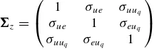
of the random disturbances, lettingzt=(ut, et, uqt)′andz=
E[ztz′t], we use
z=
⎛ ⎝ 1
σue σuuq
σue 1 σeuq
σuuq σeuq 1
⎞ ⎠,
which allows for a sufficiently general covariance structure, while imposing unit variances. Note also that our chosen co-variance matrix parameterization allows the threshold vari-able to be contemporaneously correlated with the shocks to
yt. All ourH0A-based size experiments useN=5000 replica-tions and set{α, β, ρ, φ} = {0.01,0.10,0.40,0.50}throughout. Since our initial motivation is to explore the theoretically doc-umented robustness of the limiting distribution of SupWaldAto the presence or absence of endogeneity, we consider the two scenarios given by
DGP1:{σue, σuuq, σeuq} = {−0.5,0.3,0.4},
DGP2:{σue, σuuq, σeuq} = {0.0,0.0,0.0}.
The implementation of all our Sup-based tests assumes 10% trimming at each end of the sample.
Table 1 presents some key quantiles of the SupWaldA dis-tribution (see Proposition 1) simulated using moderately small sample sizes and compares them with their asymptotic coun-terparts. Results are displayed solely for the DGP1covariance structure since the corresponding figures for DGP2were almost identical.
Looking across the different values ofcas well as the different quantiles, we note an excellent adequacy of theT =200- and
T = 400-based finite-sample distributions to the asymptotic counterpart tabulated in Andrews (1993) and Estrella (2003). This also confirms our results in Proposition 1 and provides empirical support for the fact that inferences are robust to the magnitude of c. Note that with T =200, the values of (1−
c/T) corresponding to our choices ofcin Table 1 are 0.995, 0.975, 0.950, and 0.800, respectively. Thus, the quantiles of the simulated distribution appear to be highly robust to a wide range of persistence characteristics.
Naturally, the fact that our finite-sample quantiles match closely with their asymptotic counterparts even underT=200 is not sufficient to claim that the test has good size proper-ties. For this purpose, we have computed the empirical size of the SupWaldA-based test, making use of the pvsup routine of Hansen (1997). The latter is designed to provide approximate
p-values for test statistics whose limiting distribution is as in (4). Results are presented in Table 2, which concentrates solely on the DGP1covariance structure. We initially focus on the first two
Table 1. Critical values of SupWaldA
DGP1,T=200 DGP1,T=400
c=1 c=5 c=10 c=20 c=1 c=5 c=10 c=20 ∞
2.5% 2.18 2.21 2.21 2.19 2.31 2.24 2.24 2.27 2.41
5.0% 2.53 2.52 2.57 2.50 2.65 2.63 2.62 2.63 2.75
10.0% 3.01 3.07 2.99 2.99 3.13 3.10 3.11 3.12 3.27
90.0% 10.20 10.46 10.48 10.39 10.28 10.23 10.20 10.30 10.46
95.0% 12.07 12.03 12.13 12.19 11.85 12.05 12.11 12.08 12.17
97.5% 13.82 13.76 13.85 13.84 13.74 13.57 13.91 13.64 13.71
Table 2. Size properties of SupWaldA
T=200 T=400 T=200, BOOT T=400, BOOT
2.5% 5.0% 10% 2.5% 5.0% 10% 2.5% 5.0% 10.0% 2.5% 5.0% 10.0%
c=1 2.60 4.70 8.90 2.50 4.60 9.60 3.01 6.20 11.14 3.62 5.98 11.02
c=5 2.50 4.90 9.30 2.40 4.90 9.30 2.98 6.36 11.86 3.38 6.08 11.02
c=10 2.80 4.80 9.20 2.70 5.10 9.30 3.26 6.42 12.00 3.26 5.64 10.66
c=20 2.60 4.80 9.50 2.50 5.00 9.60 3.20 6.42 11.32 3.26 6.16 11.40
left-hand panels, while the ones referred to asT =200,BOOT andT =400,BOOT are discussed later.
From the figures presented in the two left-hand panels in Table 2, we again note the robustness of the empirical size estimates of SupWaldA to the magnitude of the noncentrality parameter. Overall, the size estimates match their nominal coun-terparts quite accurately even under a moderately small sample size.
It is also interesting to compare the asymptotic approxima-tion in (4) with that occurring whenxt is assumed to follow
an AR(1), with|ρ|<1, rather than the local to unit root spec-ification we have adopted in this article. Naturally, under pure stationarity, the results of Hansen (1996,1999) apply and infer-ences can be conducted by simulating critical values from the asymptotic distribution that is the counterpart of (3) obtained under pure stationarity and following the approach outlined in the aforementioned articles. This latter approach is similar to an external bootstrap but should not be confused with the idea of obtaining critical values from a bootstrap distribution. The ob-vious question we are next interested in documenting is which approximation works better whenxt is a highly persistent
pro-cess. For this purpose, the two right-hand panels in Table 2, referred to as BOOT, present the corresponding empirical size estimates obtained using the asymptotic approximation and its external bootstrap-style implementation developed by Hansen (1996,1999) and justified by the multiplier central limit theorem (see Van der Vaart and Wellner1996). Although our comparison involves solely size properties, the above figures suggest that our nuisance-parameter-free Brownian bridge-based asymptotic ap-proximation does a good job in matching empirical sizes with nominal sizes whenρis close to the unit root frontier. Proceed-ing usProceed-ing Hansen’s (1996) approach on the other hand suggests that the procedure is mildly oversized, which does not taper off asTis allowed to increase.
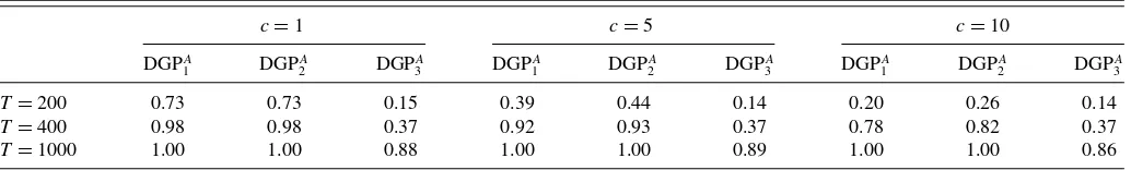
Before proceeding further, it is also important to docu-ment SupWaldA’s ability to correctly detect the presence of threshold effects via a finite-sample power analysis. Our goal here is not to develop a full theoretical and empirical power
analysis of our test statistics that would bring us well be-yond our scope but to instead give a snapshot of the abil-ity of our test statistics to lead to a correct decision under a series of fixed departures from the null. All our power-based DGPs use the same covariance structure as our size ex-periments and are based on the following configurations for {α1, α2, β1, β2, γ}in (1): DGPA1 {−0.03,−0.03,1.26,1.20,0}, DGPA2 {−0.03,0.15,1.26,1.20,0}, and DGP
A
3 {−0.03,0.25, 1.26,1.26,0}, thus covering both intercept only, slope only, and joint intercept and slope shifts. In Table 3, the figures represent correct decision frequencies evaluated as the number of times the p-value of the test statistic leads to a rejection of the null using a 2.5% nominal level.
We note from Table 3 that power converges toward 1 un-der all three parameter configurations, albeit quite slowly when only intercepts are characterized by threshold effects. The test displays good finite-sample power even underT =200 when the slopes are allowed to shift, as in DGPA1 and DGP
A
2. It is also interesting to note the negative influence of an increasing
con finite-sample power under the DGPs with shifting slopes. As expected, this effect vanishes asymptotically since even for
T ≥400, the frequencies across the different magnitudes ofc
become very similar.
4.2 TestingHB
0 :α1=α2, β1=β2=0
We next turn to the null hypothesis given by HB
0 :α1=
α2, β1=β2=0. As documented in Proposition 2, we recall that the limiting distribution of the SupWaldB statistic is no longer free of nuisance parameters and does not take a familiar form when we operate under the set of assumptions characterizing Proposition 1. However, one instance under which the limiting distribution of the SupWaldB statistic takes a simple form is when we impose the exogeneity assumption, as when consider-ing the covariance structure referred to as DGP2above. Under this scenario, the relevant limiting distribution is given by (6) and can be easily tabulated through standard simulation-based methods.
Table 3. Power properties of SupWaldA
c=1 c=5 c=10
DGPA
1 DGP
A
2 DGP
A
3 DGP
A
1 DGP
A
2 DGP
A
3 DGP
A
1 DGP
A
2 DGP
A
3
T=200 0.73 0.73 0.15 0.39 0.44 0.14 0.20 0.26 0.14
T=400 0.98 0.98 0.37 0.92 0.93 0.37 0.78 0.82 0.37
T=1000 1.00 1.00 0.88 1.00 1.00 0.89 1.00 1.00 0.86
Table 4. Critical values of SupWaldBunder exogeneity
2.5% 5% 10% 90% 95% 97.5%
c=1
T=200 2.59 3.03 3.58 11.73 13.63 15.36
T=400 2.67 3.06 3.67 11.80 13.69 15.41
T=800 2.67 3.15 3.78 11.71 13.42 15.35
c=5
T=200 2.56 3.02 3.64 11.63 13.69 15.46
T=400 2.65 3.06 3.69 11.97 13.79 15.85
T=800 2.71 3.15 3.73 11.55 13.42 15.14
For this purpose, Table 4 presents some empirical quantiles obtained usingT =200,T =400, andT =800 from the null DGPyt =0.01+ut. As can be inferred from (6) we note that
the quantiles are unaffected by the chosen magnitude ofcand appear sufficiently stable across the different sample sizes con-sidered. Viewing the T =800-based results as approximating the asymptotic distribution for instance, the quantiles obtained underT =200 andT =400 match closely with their asymp-totic counterparts.
We next turn to the more general scenario in which one wishes to testH0B within a specification that allows for endogeneity. Taking our null DGP asyt=0.01+utand the covariance
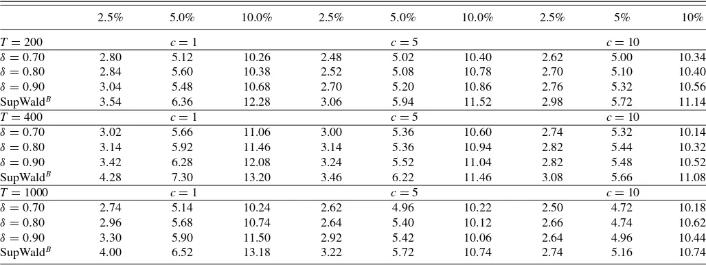
struc-ture referred to as DGP1, it is clear from Proposition 2 that using the critical values from Table 4 will lead to misleading results. This is indeed confirmed empirically with size estimates for SupWaldBlying about two percentage points above their nomi-nal counterparts (see Table 5). Using our IVX-based test statistic in (11)–(12), however, ensures that the above critical values re-main valid even under the presence of endogeneity. Results for this experiment are also presented in Table 5. Table 5 also aims to highlight the influence of the choice of theδparameter in the construction of the IVX variable (see (10)) on the size properties of the test.
Overall, we note an excellent match of the empirical sizes with their nominal counterparts. Asδ increases toward 1, it is possible to note a very slight deterioration in the size
prop-erties of SupWaldB,ivx, with empirical sizes mildly exceeding their nominal counterparts. Looking also at the power figures presented in Table 6, it is clear that asδ →1, there is a very mild-size power tradeoff that kicks in. This is perhaps not sur-prising since asδ→1, the instrumental variable starts behaving like the original nearly integrated regressor. Overall, choices of
δin the 0.7–0.8 region appear to lead to very sensible results, with almost unnoticeable variations in the corresponding size estimates. Even underδ=0.9 and looking across all configu-rations, we can reasonably argue that the resulting size proper-ties are good to excellent. Finally, the rows labeled SupWaldB clearly highlight the unsuitability of this uncorrected test statis-tic, whose limiting distribution is as in (5) and is affected by the presence of endogeneity as well as the near-integration pa-rameterc in the underlying model. In additional simulations not reported here for instance and a configuration given by {σue, σuuq, σeuq} = {−0.7,0.3,0.3},T =200,{c, δ} = {1,0.7},
we obtained empirical size estimates of 4.44%, 8.28%, and 15.04% under 2.5%, 5%, and 10% nominal sizes, respectively, for SupWaldB compared with 2.78%, 5.60%, and 10.70% for SupWaldB,ivx.
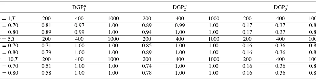
Next, we also considered the finite-sample power proper-ties of our SupWaldB,ivx statistic through a series of fixed de-partures from the null based on the following configurations for{α1, α2, β1, β2, γ}: DGPB1 {0.01,0.01,0.05,0.05,0}, DGP
B
2 {−0.03,0.25,0.05,0.05,0}, and DGPB3 {0.01,0.25,0,0,0}. Results for this set of experiments are presented in Table 6.
The above figures suggest that our modified SupWaldB,ivx statistic has good power properties under moderately large sam-ple sizes. We again note that violating the null restriction that affects the slopes leads to substantially better power properties than scenarios where solely the intercepts violate the equality constraint.
5. REGIME-SPECIFIC PREDICTABILITY OF RETURNS WITH VALUATION RATIOS
One of the most frequently explored specification in the fi-nancial economics literature has aimed to uncover the predictive
Table 5. Size properties of SupWaldB,ivxand SupWaldBunder endogeneity
2.5% 5.0% 10.0% 2.5% 5.0% 10.0% 2.5% 5% 10%
T=200 c=1 c=5 c=10
δ=0.70 2.80 5.12 10.26 2.48 5.02 10.40 2.62 5.00 10.34
δ=0.80 2.84 5.60 10.38 2.52 5.08 10.78 2.70 5.10 10.40
δ=0.90 3.04 5.48 10.68 2.70 5.20 10.86 2.76 5.32 10.56
SupWaldB 3.54 6.36 12.28 3.06 5.94 11.52 2.98 5.72 11.14
T=400 c=1 c=5 c=10
δ=0.70 3.02 5.66 11.06 3.00 5.36 10.60 2.74 5.32 10.14
δ=0.80 3.14 5.92 11.46 3.14 5.36 10.94 2.82 5.44 10.32
δ=0.90 3.42 6.28 12.08 3.24 5.52 11.04 2.82 5.48 10.52
SupWaldB 4.28 7.30 13.20 3.46 6.22 11.46 3.08 5.66 11.08
T=1000 c=1 c=5 c=10
δ=0.70 2.74 5.14 10.24 2.62 4.96 10.22 2.50 4.72 10.18
δ=0.80 2.96 5.68 10.74 2.64 5.40 10.12 2.66 4.74 10.62
δ=0.90 3.30 5.90 11.50 2.92 5.42 10.06 2.64 4.96 10.44
SupWaldB 4.00 6.52 13.18 3.22 5.72 10.74 2.74 5.16 10.74
Table 6. Power properties of SupWaldB,ivx
DGPB
1 DGPB2 DGPB3
c=1,T 200 400 1000 200 400 1000 200 400 1000
δ=0.70 0.81 0.97 1.00 0.89 0.99 1.00 0.17 0.37 0.87
δ=0.80 0.89 0.99 1.00 0.94 1.00 1.00 0.17 0.37 0.87
c=5,T 200 400 1000 200 400 1000 200 400 1000
δ=0.70 0.71 1.00 1.00 0.85 1.00 1.00 0.16 0.36 0.87
δ=0.80 0.79 1.00 1.00 0.89 1.00 1.00 0.16 0.36 0.87
c=10,T 200 400 1000 200 400 1000 200 400 1000
δ=0.70 0.51 1.00 1.00 0.74 1.00 1.00 0.16 0.36 0.87
δ=0.80 0.58 1.00 1.00 0.78 1.00 1.00 0.16 0.36 0.86
power of valuation ratios such as DYs for future stock returns via significance tests implemented on simple linear regressions link-ingrt+1to DYt. The econometric complications that arise due to
the presence of a persistent regressor, together with endogeneity issues, have generated a vast methodological literature aiming to improve inferences in such models, commonly referred to as predictive regressions (e.g., Valkanov2003; Lewellen2004; Campbell and Yogo2006; Jansson and Moreira2006; Ang and Bekaert2007, among numerous others).
Given the multitude of studies conducted over a variety of sample periods, methodologies, data definitions, and frequen-cies, it is difficult to extract a clear consensus on predictabil-ity. From the recent analysis of Campbell and Yogo (2006), there appears to be statistical support for some very mild DY-based predictability, with the latter having substantially declined in strength post 1995 (see also Lettau and Van Nieuwerburgh 2008). Using monthly data over the 1946–2000 period, Lewellen (2004) documented a rather stronger DY-based predictability using a different methodology that was mainly concerned with small-sample bias correction. See also Cochrane (2008) for a more general overview of this literature.
Our goal here is to reconsider this potential presence of pre-dictability through our regime-based methodology focusing on the DY predictor. More specifically, using growth in industrial production as our threshold variable proxying for aggregate macro conditions, our aim is to assess whether the data sup-port the presence of regime-dependent predictability induced by good versus bad economic times. Theoretical arguments justify-ing the possible existence of episodic instability in predictability have been alluded to in the theoretical setting of Menzly, San-tos, and Veronesi (2004), and more recently, Henkel, Martin, and Nardari (2009) explored the issue empirically using Bayesian methods within a Markov switching setup. We will show that our approach leads to a novel view and interpretation of the predictability phenomenon and that its conclusions are robust across alternative sample periods. Moreover, our findings may provide an explanation for the lack of robustness to the sample period documented in existing work under linearity. An alterna-tive strand of the recent predicalterna-tive regression literature, or more generally the forecasting literature, has also explored the issue of predictive instability through the allowance of time variation via structural breaks and the use of recursive estimation tech-niques. A general message that has come out from this research is the omnipresence of model instability and the important in-fluence of time variation on forecasts (see Rossi2005,2006;
Rapach and Wohar 2006; Timmermann2008, among others). Our own research is also motivated by similar concerns but fo-cuses on explicitly identifying predictability episodes induced by a particular variable such as a business cycle proxy.
Our analysis will be based on the same CRSP (Center for Research in Security Prices) dataset as the one considered in the vast majority of predictability studies (value-weighted re-turns for NYSE, AMEX, and NASDAQ). Throughout all our specifications, the dividend yield is defined as the aggregate dividends paid over the last 12 months divided by the market capitalization and is logged throughout (LDY thereafter). For robustness considerations, we will distinguish between returns that include dividends and returns that exclude dividends. Fi-nally, using the 90-day T-bills (Treasury bills), all our inferences will also distinguish between raw returns and their excess coun-terparts. Following Lewellen (2004), we will restrict our sample to the post-war period. We will concentrate solely on monthly data since the regime-specific nature of our models would make yearly or even quarterly data-based inferences less reliable due to the potentially very small size of the sample. We will sub-sequently explore the robustness of our results to alternative sample periods.
Looking first at the stochastic properties of the DY predictor over the 1950M1–2007M12 period, it is clear that the series is highly persistent, as judged by a first-order sample auto-correlation coefficient of 0.991. A unit root test implemented on the same series unequivocally fails to reject the unit root null. The industrial production growth series is stationary as ex-pected, displaying some very mild first-order serial correlation and clearly conforming to our assumptions aboutqtin (1)–(2).
Before proceeding with the detection of regime-specific pre-dictability, we start by assessing return predictability within a linear specification, as has been done in the existing litera-ture. Results across both raw and excess returns are presented in Table 7, with VWRETD denoting the returns inclusive of dividends and VWRETX denoting the returns ex-dividends. The columns named as p andpHAC refer to the standard and HAC (heteroscedasticity and autocorrelation consistent)-based
p-values.
The coefficient estimates of Table 7 refer to the OLS (ordi-nary least squares) estimates of βDYin the regression rt+1=
α+βDYLDYt+ut+1. Focusing first on the VWRETD series, our results conform with the consensus that predictability has been vanishing from the late 1980s onward (for instance, see Campbell and Yogo 2006). The remaining p-values suggest
Table 7. Linear predictabilityrt+1=αDY+βDYLDYt+ut+1
VWRETD βˆDY pHAC p R2 VWRETX βˆDY pHAC p R2
1950–2007 0.010 0.011 0.008 0.9% 1950–2007 0.008 0.054 0.046 0.4%
1960–2007 0.010 0.056 0.037 0.6% 1960–2007 0.008 0.142 0.110 0.3%
1970–2007 0.009 0.069 0.056 0.6% 1970–2007 0.007 0.170 0.148 0.2%
1980–2007 0.011 0.059 0.042 0.9% 1980–2007 0.009 0.131 0.103 0.5%
1990–2007 0.014 0.153 0.105 0.8% 1990–2007 0.001 0.207 0.152 0.5%
Excess Excess
1950–2007 0.009 0.025 0.019 0.7% 1950–2007 0.007 0.102 0.087 0.3%
1960–2007 0.007 0.210 0.169 0.2% 1960–2007 0.004 0.417 0.372 0.0%
1970–2007 0.006 0.269 0.240 0.1% 1970–2007 0.004 0.665 0.479 0.0%
1980–2007 0.007 0.253 0.208 0.2% 1980–2007 0.005 0.439 0.392 0.0%
1990–2007 0.013 0.198 0.138 0.6% 1990–2007 0.011 0.263 0.196 0.0%
some mild predictability, especially when considering the entire 1950–2007 sample range. Interestingly, as we switch from raw to excess returns, the picture changes considerably, with most
p-values strongly pointing toward the absence of any predictabil-ity. Given thesep-value magnitudes, it is difficult to conceive that any methodological improvements may reverse the big pic-ture. Also worth pointing out is the fact that a conventional test for heteroscedasticity implemented on the above specifications failed to reject the null of no heteroscedasticity. This is partic-ularly reassuring since one of our assumptions leading to our theoretical results in Propositions 1 and 2 ruled out the presence of heteroscedasticity.
Next, focusing on the returns that exclude dividend payments, it is again the case that withp-values as high as 0.665, the null of no predictability cannot be rejected. Results appear to also be robust across different starting periods, except perhaps under the full 1950–2007 range, under which we note a mild rejection of the null. It is also important to note that all results were robust across HAC versus non-HAC standard errors. This latter point is particularly important since our assumptions surrounding (1)– (2) rule out serial correlation and heteroscedasticity inut.
Overall, the above linearity-based results corroborate the view that predictability is at best mildly present and its strength ap-pears to have declined. Perhaps more importantly, Table 7 also suggests that one should be particularly cautious and worry about robustness considerations when assessing DY-induced predictability of returns since findings may be extremely sen-sitive to data definitions, frequency, and chosen sample period. At this stage, it is also important to reiterate that our analysis in Table 7 is mainly meant to provide a comparison benchmark for our subsequent regime-based inferences rather than reverse findings from the existing literature. This is also the reason why we do not explore outcomes based on alternative methodologies, as developed in the recent econometric literature.
The fact that numerous studies documented a decline in predictability characterizing the 1990s could also be due to the fact that predictability kicks in during particular economic episodes. Table 8 presents the results of our tests of the hypothe-sesHB
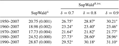
0 :α1=α2, β1=β2=0 andH0A:α1=α2, β1=β2as applied to the VWRETD series (∗indicates rejection at 2.5%). Since results for the return series that exclude dividends as well as their excess counterparts were both qualitatively and quanti-tatively similar, in what follows, we concentrate solely on the VWRETD series.
The evidence presented in Table 8 comfortably points toward the presence of regime-specific predictability since bothHA
0 and
HB
0 are strongly rejected. We also note that inferences based on SupWaldB,ivx appear robust to alternative choices of δ in the construction of the IVX variable. It is also interesting to note that unlike the linear case, inferences appear to be robust to the starting period. One should be cautious, however, when interpreting inferences such as the ones based on the 1990– 2007 period due to sample size limitations, which are further exacerbated when fitting a threshold specification.
Recalling that theR2’s characterizing the various linear speci-fications were clustered around values close to zero (see Table 7), it is also useful to highlight the remarkable jump in goodness of fit in our proposed threshold model presented in (15). Our results strongly point toward the presence of very strong predictabil-ity duringbad timeswhen the growth in industrial production (IP) (variable IPt=ln(IPt/IPt−1)) is negative, while no or very weak predictability during expansionary periods or normal times. More specifically, over the 1950–2007 period, we have
ˆ
rt+1 = ⎧ ⎪ ⎪ ⎪ ⎨ ⎪ ⎪ ⎪ ⎩
0.1606(0.0357)+0.0441(0.0107)LDYt
IPt ≤ −0.0036,R12=17.47%,N1=131 0.0135(0.0161)+0.0010(0.0045)LDYt
IPt >−0.0036,R22=0.00%,N2=564, (15)
with a jointR2of 3.88%. Estimated standard errors are in paren-theses. Besides being interesting in its own right, this result may also help explain the conflicting results obtained in the recent literature where the samples considered included or excluded data on the late 1990s and 2000s, a period with few reces-sions. Even with the reduction in the sample size, it is quite
Table 8. Regime-specific predictability
SupWaldB,ivx
SupWaldA δ
=0.7 δ=0.8 δ=0.9
1950–2007 20.75 (0.001) 26.75∗ 28.87∗ 30.21∗ 1960–2007 18.98 (0.002) 23.24∗ 23.40∗ 23.46∗ 1970–2007 17.73 (0.004) 21.64∗ 21.82∗ 21.77∗ 1980–2007 24.52 (0.000) 27.73∗ 28.60∗ 28.96∗ 1990–2007 28.87 (0.000) 29.52∗ 30.18∗ 31.10∗
remarkable that the goodness of fit can jump from a magnitude close to zero to about 17% in one subset. Overall, our results strongly support DY-based predictability in U.S. returns but oc-curring solely duringbad times. Note, for instance, that more than half of the periods during which IPt ≤ −0.0036
coin-cide with the NBER (National Bureau of Economic Research) recessions. The strength of this predictability is very strong and unlikely to be sensitive to the methodology or our assumptions. Interestingly and through a different methodology, our findings about the presence of strong return predictability during bad times also corroborate the findings in Henkel et al. (2009). Us-ing Bayesian inference techniques on a Markov switchUs-ing VAR (vector autoregression) setup in which they consider multiple predictors in addition to the DY, the authors document a sub-stantial jump in predictive strength of variables such as DY, short-term rates, term structure, etc., during recessions.
6. CONCLUSIONS
The goal of this article was to develop inference methods use-ful for detecting the presence of regime-specific predictability in predictive regressions. We obtained the limiting distributions of a series of Wald statistics designed to test the null of linearity versus threshold-type nonlinearity and the joint null of linear-ity and no predictabillinear-ity. One important feature of the limiting distribution that arises in the first case is the fact that it does not depend on any unknown nuisance parameters, thus making it straightforward to use. This is an unusual occurrence in this literature, where under a purely stationary framework (as op-posed to a nearly integrated one), it is well known that limiting distributions typically depend on unknown population moments of the underlying models.
Our empirical application also leads to the interesting result that U.S. return series are clearly predictable using valuation ratios such as DY, but this predictability kicks in solely during bad times and would therefore be masked in studies that operate within linear specifications.
Finally, some important extensions to the present work are worth mentioning. A useful extension we are currently considering involves introducing long-horizon variables into (1)–(2). This would offer an interesting parallel to the linear predictive regression literature, which has often distinguished long- versus short-horizon predictability. Other important extensions include extending (1)–(2) to allow for more than two regimes, following some of the methods developed in Gonzalo and Pitarakis (2002), while further statistical properties (e.g., confidence intervals) of objects such as the estimated threshold parameter may be explored using the subsampling methodology of Gonzalo and Wolf (2005).
A key assumption under which we have operated ruled out heteroscedasticity and serial correlation inut. As our empirical
application has documented however, our results can continue to be extremely useful despite this limitation. This restriction is in fact the norm rather than the exception in any work that introduced nonlinearities parametrically or nonparametrically in models that contain persistent variables. Albeit challenging, we expect future work to also be directed toward tackling these issues.
APPENDIX: PROOFS
Lemma 1. Under Assumptions 1 and 2 and as T →
∞, we have (a)
mixing with the same mixing numbers as qt. The result then
follows from a suitable law of large numbers (see White2001, secs. 3.3– 3.4). (b)–(e) Under our Assumptions 1 and 2, the results follow directly from lemma 3.1 in Phillips (1988). (f) LettingXT ,t =xt/
some p≥4, we can make use of the strong approxima-tion result supr∈[0,1]|XT(r)−Kc(r)| =op(T−a), with a=
The above then leads to
1
holding uniformly ∀λ∈. Finally, given that supr∈[0,1]|XT(r)| =Op(1), together with the fact that the
result in (a) also holds uniformly overλ(see lemma 1 in Hansen 1996), we have supλ|
implying the required result. (g) follows identical lines to the proof of (f). (h)–(i) Since our assumptions satisfy their assumption 2, the result in (h) is theorem 1 of Caner and Hansen (2001), while our result in (i) follows along the same lines as theorem 2 of Caner and Hansen (2001).
Proof of Proposition 1. It is initially convenient to
reformu-and using Lemma 1, we have the following weak convergence results: Looking at each component separately, settingσu2=1 for sim-plicity and no loss of generality and using Lemma 1, we have
DT−1X1′u=
The above now allows us to formulate the limiting behavior of
DT−1X′
straightforwardly through the use of the CMT and standard algebra.
Proof of Proposition 2. We rewrite our most general un-restricted specification in (1) as y =α1I1+β1x1+α2I2+
within this alternative parameterization,HA
0 :η=0 andH0B :
η=0, β=0. Next, consider a most general (MG) model containing (1 x X2)=(X X2), a partially restricted (PR) version containing X=(1 x), and a fully restricted (FR) version containing the vector of 1’s. From standard projec-tion algebra, the sum of squared errors corresponding to each specification are SSEMG=y′MX,X2y, SSEP R=y′MXy, and
SSEF R=y′M1y, whereMX =I −X(X′X)−1X′andMX,X2 =
MX−MXX2(X′2MXX2)−1X2′MX. It now trivially follows that
we can write the Wald statistics corresponding to each hy-pothesis as WA can now immediately be observed that WB
T(λ)=WTA(λ)+
( ˆσ2
lin/σˆu2)WT(β=0). Under the null hypothesis, ( ˆσlin2/σˆu2) p
→1 and therefore in large samples,WB
T(λ)≈WT(β =0)+WTA(λ)
and supλWTB(λ)≈WT(β =0)+supλWTA(λ), as required. To
obtain the limiting distribution in (5), it now suffices to use the results presented in Lemma 1, together with the CMT along lines identical to those in the proof of Proposition 1.
Proof of Proposition 3. Our result in (13) follows directly from (11)–(12), theorem 3.8 in PM09 (p. 14), Lemma 1, Propo-sition 1, and the use of the CMT. Note that theorem 3.8 in PM09 has been obtained within a model with no fitted intercept; how-ever, Stamatogiannis (2010, theorem 4.2, p. 154) and Kostakis et al. (2010) also established its validity in the more general setting that includes a constant term and a predictive regression setting identical to our specification in (7) and thus leading to our own result.
SUPPLEMENTARY MATERIALS
Appendix:File providing additional Monte Carlo simulations and further details on some of the proofs.
ACKNOWLEDGMENTS
J. Gonzalo thanks the Spanish Ministerio de Ciencia e Innova-cion, grants SEJ2007-63098, ECO2010-19357, CONSOLIDER 2010 (CSD 2006-00016), DGUCM (Community of Madrid) grant EXCELECON S-2007/HUM-044 and Bank of Spain (ER program) for partially supporting this research. J. Pitarakis thanks the ESRC for partially supporting this research through an individual research grant RES-000-22-3983. Both authors are grateful to Grant Hillier, Tassos Magdalinos, Peter Phillips, and Peter Robinson for very useful suggestions and helpful discussions. Detailed comments and feedback from the editor, associate editor and two anonymous referees are also grate-fully acknowledged. Last but not least, we also thank seminar participants at Queen-Mary, LSE, Southampton, Exeter, Manch-ester, and Nottingham universities, the ESEM 2009 meetings in
Barcelona, the SNDE 2010 meeting in Novara, and the 2010 CFE conference in London for useful comments. All errors are our own responsibility.
[Received March 2010. Revised June 2011.]
REFERENCES
Andrews, D. W. K. (1993), “Tests for Parameter Instability and Struc-tural Change With Unknown Change Point,” Econometrica, 61, 821– 856. [232,234]
Ang, A., and Bekaert, G. (2007), “Stock Return Predictability: Is It There?,”
Review of Financial Studies, 20, 651–707. [230,237]
Bandi, F., and Perron, B. (2008), “Long-Run Risk-Return Trade-Offs,”Journal of Econometrics, 143, 349–374. [229]
Campbell, J. Y., and Yogo, M. (2006), “Efficient Tests of Stock Re-turn Predictability,” Journal of Financial Economics, 81, 27–60. [229,230,231,237,237]
Caner, M., and Hansen, B. E. (2001), “Threshold Autoregression With a Unit Root,”Econometrica, 69, 1555–1596. [230,232,239]
Cavanagh, C. L., Elliott, G., and Stock, J. H. (1995), “Inference in Models With Nearly Integrated Regressors,”Econometric Theory, 11, 1131–1147. [230,231]
Chan, N. (1988), “The Parameter Inference for Nearly Nonstationary Time Se-ries the Parameter Inference for Nearly Nonstationary Time SeSe-ries,”Journal of the American Statistical Association, 83, 857–862. [230]
Cochrane, J. H. (2008), “The Dog That Did Not Bark: A Defense of Return Predictability,”Review of Financial Studies, 21, 1533–1575. [229,237] Elliott, G. (1998), “On the Robustness of Cointegration Methods When
Regres-sors Almost Have Unit Roots,”Econometrica, 66, 149–158. [233] Estrella, A. (2003), “Critical Values and P Values of Bessel Process
Distribu-tions: Computation and Application to Structural Break Tests,”Econometric Theory, 19, 1128–1143. [232,234]
Gonzalo, J., and Pitarakis, J. (2002), “Estimation and Model Selection Based In-ference in Single and Multiple Threshold Models,”Journal of Econometrics, 110, 319–352. [239]
Gonzalo, J., and Wolf, M. (2005), “Subsampling Inference in Threshold Au-toregressive Models,”Journal of Econometrics, 127, 201–224. [239] Hansen, B. E. (1996), “Inference When a Nuisance Parameter Is Not Identified
Under the Null Hypothesis,”Econometrica, 64, 413–430. [232,235,239] ——— (1997), “Approximate Asymptotic P-Values for Structural Change
Tests,” Journal of Business and Economic Statistics, 15, 60–67. [232,234]
——— (1999), “Testing for Linearity,”Journal of Economic Surveys, 13, 551– 576. [235]
Henkel, S. J., Martin, J. S., and Nardari, F. (2009), “Time-Varying Short-Horizon Return Predictability,” AFA 2008 New Orleans Meetings Paper [on-line]. Available athttp://ssrn.com/abstract=1101944. [237,239]
Jansson, M., and Moreira, M. J. (2006), “Optimal Inference in Regression Models With Nearly Integrated Regressors,”Econometrica, 74, 681–714. [229,230,231,237]
Kostakis, A., Magdalinos, A., and Stamatogiannis, M. (2010), “Econometric In-ference for Stock Return Predictability,” unpublished manuscript, University of Nottingham, UK. [233,240]
Lettau, M., and Van Nieuwerburgh, S. (2008), “Reconciling the Re-turn Predictability Evidence,” Review of Financial Studies, 21, 1607– 1652. [229,237]
Lewellen, J. (2004), “Predicting Returns With Financial Rations,”Journal of Financial Economics, 74, 209–235. [229,237,237]
Menzly, L., Santos, T., and Veronesi, P. (2004), “Understanding Predictability,”
Journal of Political Economy, 112, 1–47. [237]
Park, J. Y., and Phillips, P. C. B. (1988), “Statistical Inference in Regressions With Integrated Processes: Part 1,”Econometric Theory, 4, 468–497. [232] Petruccelli, J. D. (1992), “On The Approximation of Time Series by Threshold
Autoregressive Models,”Sankhya,Series B, 54, 54–61. [230]
Phillips, P. C. B. (1988), “Regression Theory for Near-Integrated Time Series,”
Econometrica, 56, 1021–1043. [231,239]
——— (1998), “New Tools for Understanding Spurious Regressions,” Econo-metrica, 66, 1299–1325. [239]
Phillips, P. C. B., and Hansen, B. E. (1990), “Statistical Inference in Instrumental Variables Regression With I(1) Process,”Review of Economic Studies, 57, 99–125. [233]
Phillips, P. C. B., and Magdalinos, A. (2007), “Limit Theory for Moderate Deviations From a Unit Root Under Weak Dependence,”Journal of Econo-metrics, 136, 115–130. [239]
——— (2009), “Econometric Inference in the Vicinity of Unity,” CoFie Work-ing Paper No. 7, SWork-ingapore Management University, SWork-ingapore. [233] Pitarakis, J. (2008), “Threshold Autoregressions With a Unit Root: Comment,”
Econometrica, 76, 1207–1217. [230,232]
Rapach, D. E., and Wohar, M. E. (2006), “Structural Breaks and Predictive Regression Models of Aggregate U.S. Stock Returns,”Journal of Financial Econometrics, 4, 238–274. [237]
Rossi, B. (2005), “Optimal Tests for Nested Model Selection With Underlying Parameter Instability,”Econometric Theory, 21, 962–990. [233,237] ——— (2006), “Are Exchange Rates Really Random Walks? Some Evidence
Robust to Parameter Instability,”Macroeconomic Dynamics, 10, 20–38. [237]
Saikkonen, P. (1991), “Asymptotically Efficient Estimation of Cointegrating Regressions,”Econometric Theory, 7, 1–21. [233]
——— (1992), “Estimation and Testing of Cointegrated Systems by an Autore-gressive Approximation,”Econometric Theory, 8, 1–27. [233]
Stamatogiannis, M. P. (2010), “Econometric Inference in Mod-els With Nonstationary Time Series,” Ph.D. Dissertation, De-partment of Economics, University of Nottingham. Available at
http://etheses.nottingham.ac.uk/1950/1/StamatogiannisThesis2010.pdf
[233,240]
Timmermann, A. (2008), “Elusive Return Predictability,”International Journal of Forecasting, 24, 1–18. [237]
Valkanov, R. (2003), “Long-Horizon Regressions: Theoretical Results and Ap-plications,”Journal of Financial Economics, 68, 201–232. [229,237] Van der Vaart, J., and Wellner, J. (1996), Weak Convergence and
Em-pirical Processes: With Applications to Statistics, New York: Springer-Verlag. [235]
White, H. (2001), Asymptotic Theory for Econometricians (2nd rev. ed.), New York: Academic Press. [239]