ON FINDING
THE FUNDAMENTAL DOMINANT WEIGHTS OF A ROOT SYSTEM
By Hendra Gunawan
Department of Mathematics, Institut Teknologi Bandung
Jalan Ganesha 10 Bandung 40132, Indonesia
Abstract. This note offers a formula which can be used as an alternative method of finding the fundamental dominant weights of a root system, as suggested in [3]. We explain how the formula actually works and verify the fundamental dominant weights of root systems of type A – G.
Introduction
Almost all symbols and terminology we use here are the same as in [4, Ch. III]. Let Φ be a root system of rank l. Fix ∆ ={α1, . . . , αl} to be a base of Φ. Relative to ∆, denote by Φ+
the set of positive roots, whose members are of the form α= l
P
j=1
kj(α)αj where the
kj(α)’s are all nonnegative integers. Denote byδthe special element, namelyδ = 12 P
α∈Φ+
α.
Now let{λ1, . . . , λl}be the dual basis, for whichhλj, αki=δjk, j, k∈ {1, . . . , l}. Then we
know that δ= l
P
j=1
λj, showing that δ is a dominant weight.
Let us fix any j0 ∈ {1, . . . , l} and put Φ +
0 = {α ∈ Φ + : k
j0(α) = 0}. Then Φ0 = Φ+0 ∪(−Φ
+
0) forms a root system of rank l −1. Φ +
0 is obviously the corresponding set of positive roots relative to the base ∆0 = {αj : j 6= j0}. Let δ0 = 12 P
α∈Φ+0
α and set
δ1 =δ−δ0. (Note that δ0 depends on the choice ofj0, and so does δ1.) One may observe that δ1 is actually the projection of δ on λj0. Moreover, as announced in [3], we have the following result.
Theorem. λj0 = δ1
hδ1,αj0i.
The theorem offers a formula which can be used as an alternative method of finding the fundamental dominant weightλj0 for any givenj0 ∈ {1, . . . , l}. Using this formula, we can
find one particular fundamental dominant weight without worrying about the others. It is —in this case— less labor than employing the Cartan matrix (where we have to invert the matrix). Note, however, that the formula is useful only when we knowδ and δ0 (so we can find δ1).
We give here a shorter proof of the theorem. We also explain how to find δ1, and then compute and verify the fundamental dominant weights λj0, j0 ∈ {1, . . . , l}, of root systems of type A – G.
1. Proof of the Theorem
The theorem follows from the lemma below, which we have stated before.
Lemma. δ1 = 1
2hδ, λj0iλj0.
Proof. For eachj ∈ {1, . . . , l}, setλ∗
j =λj−12hλj, λj0iλj0. We observe that forj, k 6=j0,
hλ∗j, αki=hλj, αki − 1
2hλj, λj0ihλj0, αki=hλj, αki=δjk,
that is, {λ∗j :j 6=j0} is the dual basis relative to ∆0 (see [3] for more details). From this
and the fact that λ∗j0 = 0, we have δ0 = l
P
j=1
λ∗j, and accordingly
δ1 =δ−δ0
= l
X
j=1
λj − l
X
j=1
λ∗j
= 1 2
l
X
j=1
hλj, λj0iλj0
= 1 2h
l
P
j=1
λj, λj0iλj0
= 1
2hδ, λj0iλj0, proving the lemma. ⊔⊓
Now we prove the theorem.
Proof of the Theorem. Using the above lemma, we have
hδ1, αj0i= 1
2hδ, λj0ihλj0, αj0i= 1
Hence we obtain that
δ1 =hδ1, αj0iλj0
or
λj0 = δ1 hδ1, αj0i
,
as stated. ⊔⊓
2. Finding δ1
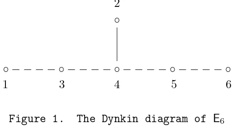
We use the following technique to find δ1. (In [2], the same technique is used for a different purpose.) Suppose, for example, Φ is a root system of type E6, whose Dynkin diagram is as follows.
2 ◦
◦ − − − − ◦ − − − − ◦ − − − − ◦ − − − − ◦
1 3 4 5 6
Figure 1. The Dynkin diagram of E6
Remove the j0-th vertex from the diagram to obtain a new diagram, which in general will be a union of Dynkin diagrams. For example, if we remove the 4th vertex, then we get a diagram for A2 ∪ A1 ∪ A2. The resulting diagram is the Dynkin diagram of the root system Φ0. Keeping in mind the roots associated with the vertices, we determine the weightδ0, using available formulae. We then easily computeδ1 =δ−δ0. For our example, by removing the 4th vertex we get
δ0 =α1+ 1
2α2+α3+α5+α6.
We know that
δ = 8α1+ 11α2+ 15α3+ 21α4+ 15α5+ 8α6,
and therefore
δ1 = 7α1+ 21
For root systems of type A – G, we use the (ordered) bases as in [4, pp. 64-65]. With respect to these bases, explicit formulae for the weight δ are obtainable (see, for example, [1]).
vertex from the Dynkin diagram will yield a diagram for Aj0−1 ∪ Al−j0. Accordingly we
get δ0 = 12 the j0-th vertex from the Dynkin diagram will yield a diagram for Aj0−1∪ Cl−j0. So we
For convenience, we abbreviate Pl
j=1
kjαj by (k1, . . . , kl).
2.5E6,E7, andE8. In typeE6, we haveδ = (8,11,15,21,15,8), as mentioned before. Below are the δ0’s and δ1’s obtained by removing the j0-th vertex from the Dynkin diagram.
j0 δ0 δ1 by removing the j0-th vertex from the Dynkin diagram are listed below.
j0 δ0 δ1 the Dynkin diagram we obtain the following list.
4 (1,1
2,1,0,2,3,3,2) (45, 135
2 ,90,135,108,81,54,27) 5 (2,2,3,3,0,32,2,32) (44,66,88,132,110,1652 ,55, 552 ) 6 (4,5,7,9,5,0,1,1) (42,63,84,126,105,84,56,28) 7 (8,11,15,21,15,8,0,12) (38,57,76,114,95,76,57,572 ) 8 (17,492 ,33,48, 752 ,26,272 ,0) (29,872 ,58,87,1452 ,58,872 ,29)
2.6 F4. Here we have δ = (8,15,21,11). Removing the j0-th vertex from the Dynkin diagram will give the following result.
j0 δ0 δ1
1 (0,3,5,3) (8,12,16,8) 2 (1
2,0,1,1) ( 15
2,15,20,10) 3 (1,1,0,1
2) (7,14,21, 21
2 ) 4 (5
2,4, 9
2,0) ( 11
2,11, 33
2 ,11)
2.7 G2. The special element is δ = (5,3). Removing either vertex from the Dynkin diagram will yield a diagram for A1. When the 1st vertex is removed, we get δ0 = (0,1
2) and δ1 = (5,52). When the 2nd vertex is removed, we get δ0 = (12,0) and δ1 = (92,3).
3. Computing λj0
Having foundδ1, we only need to divide it byhδ1, αj0ito getλj0. Knowing the Cartan integers hαi, αji makes it easy to calculate hδ1, αj0i.
Below are the values of hδ1, αj0i for root systems of type A – G.
For typeA – D, we have the following result.
Al (l ≥1) : hδ1, αj0i= 1
2(l+ 1), j0 = 1, . . . , l. Bl (l ≥2) : hδ1, αj0i=
½1
2(2l−j0), j0 = 1, . . . , l−1;
l, j0 =l.
Cl (l≥3) : hδ1, αj0i= 1
2(2l−j0+ 1), j0 = 1, . . . , l. Dl (l ≥4) : hδ1, αj0i=
½1
2(2l−j0−1), j0 = 1, . . . , l−2;
For type E – G, we have the following result. (The values of hδ1, αj0i are listed as j0
increases from 1 to l.)
E6 : 6,11 2 ,
9 2,
7 2,
9 2,6. E7 : 17
2 ,7, 11
2 ,4,5, 13
2 ,9. E8 : 23
2 , 17
2 , 13
2, 9 2,
11 2,7,
19 2 ,
29 2.
F4 : 4,5 2,
7 2,
11 2 . G2 : 5
2, 3 2.
The above results clearly verify the fundamental dominant weights of root systems of type A – G listed in [4, p. 69].
References
[1] J.-P. Antoine and D. Speiser, Characters of irreducible representations of the simple groups. II. Applications to classical groups, J. Mathematical Physics, 5(1964), 1560-1572. [2] M. Cowling and C. Meaney, On a maximal function on compact Lie groups, Trans. Amer. Math. Soc., 315(1989), 811-822.
[3] H. Gunawan,A generalization of maximal functions on compact semisimple Lie groups, Pac. J. Math., 156(1992), 119-134.