Application of Discrete Discriminant Analysis In Public Health Phenomenon A Safe-Motherhood Study

In Public Health Phenomenon A

Safe-Motherhood Study

Kuntoro Kuntoro

1

_{, Rahmah Indawati}

1

_{, Diah Indriani}

1

_{, Arief Wibowo}

1

1_{Department of Biostatistics and Population Study, Airlangga University School of Public}

Health, Surabaya 60115, Indonesia. kuntoro1@indo.net.id, kuntoro2@yahoo.com; 1; 1; 1

Abstract

Linear discriminant analysis is used widely in medical sciences since most dis-criminator variables have interval and ratio scale besides multivariate normal and unknown but equal dispersion and covariance matrices assumptions are met. How-ever, in public health sciences most discriminator variables have ordinal and nominal scales so that linear discriminant analysis is not recommended. When ordinal and nominal scales are categorized into positive and negative, a discrete discriminant analysis is prefered.

The data of safe-motherhood collected by Kuntoro et al. (1999) that include group assignment (mother : dead, alive), five discriminator variables (x), place of delivery baby, person who delivered baby, antenatal care, place of antenatal care, and referal services obtained. Allocation of a new observation x into Group 1 (dead) if ˆ

g1(x)>ˆg2(x)and into Group 2 (alive) if ˆg1(x)<ˆg2(x).

The results showed that in the beginning of group assignment there were 65 mothers who were dead and 976 mothers who were alive. Discrete discriminant analysis gives 93.95% correct classification, while linear discriminant analysis, logistic regression analysis, and neural network discriminant analysis give respectively 86.6%, 93.76% and 93.76%.

It is concluded that discrete discriminant analysis seems to be the most effec-tive in discriminating individuals into groups when the discriminator variables are dichotomously categorical.

Keywords: correct classification, discriminator, group assignment

1

Introduction

Determining the procedure for classifying an individual who has a number of physical and laboratory examination results falls into a disease or non disease under study is important in medical sciences. This procedure is required by a medical professional for selecting the medical action when an individual falls into a disease group under study. This procedure is commonly calledcut-off_.

There are several statistical methods related tocut-off_{, one of them is linear}

discrimi-nant analysis. It is used widely in medical sciences since most discriminator variables have interval and ratio scale besides multivariate normal and unknown but equal dispersion and covariance matrices assumptions are met.

In public health sciences as well as in medical sciences the procedure mentioned above is also required by a public health professional for the same purpose. Unlike in medical sciences whose variables of interest have interval or ratio scales, in public health sciences whose variables of interest have ordinal and nominal scales. In this case, a linear discrim-inant analysis is not recommended. When ordinal and nominal scales are categorized into positive and negative, a discrete discriminant analysis is prefered.

2

Basic Concepts

2.1

Discrete Discriminant Analysis

Consider random variables X1, X2, . . . , Xp. It is assumed that each random variable has

at most a finite number of distinct values s1, s2, . . . , sp. Moreover, the product represents

the set of all possible values. Furthermore, xdenotes a particular realization of X. The underlying distribution within each subpopulation is assumed to be multinomial. In the case of two groups, let the class conditional density in Gi befi and the prior probability

of membership be Pi where i = 1,2. A new observation x will be assigned into G1 if

P1f1(x)> P2f2(x) and into G2 if P1f1(x)< P2f2(x). The assignment is done randomly if P1f1(x) = P2f2(x) [2] Let P1f1(x) be a discriminant score, its value is denoted by

g1(x). Let n observations be samples from the combined population, and let ni(x) be

the number from Gi having measurment x. Hence, n = Px

P

ini(x). Let Pin_ni and

ˆ

fi(x) = _nnnix

i be respectively nonparametric estimates of prior probabilities and the class

conditional densities that yield sample-based estimates of the discriminant scores, [2] The sample-based rule can be described as follows : AssignxtoG1 if ˆg1(x)>g2ˆ(x) and toG2

if ˆg1(x)<g2ˆ(x) and allocate randomly if ˆg1(x) = ˆg2(x) [2]

2.2

Linear Discriminant Analysis

LetDi =b1x1i+b2x2i+...+bpxpibe standardized linear discriminant function, where

Diis score discriminant for individuali, biis discriminant coefficient, wherei= 1,2, . . . , p

and xi is discriminator variable, wherei= 1,2, . . . , p. Let

¯

D1+ ¯D2

2 be a cut-off, where ¯D1

and ¯D2 are the means of discriminant scores in respectively group 1 and group 2. The rule of classification: If ¯D1>D2¯ , an individual with a given value ofxi is assigned toG1

if his/her discriminant score Di > cut-off and to G2 if his/her discriminant score Di <

cut-off. If ¯D1 <D2¯ , an individual with a given value of xi is assigned to G1 if his/her

discriminant score<cut-off and toG2if his/her discriminant score>cut-off [3, 4]

2.3

Logistic Regression Analysis

Logistic Regression Model relates a number of independent variables whose scales can be nominal, ordinal, interval and ratio and a dependent variabel whose scale is nominal cat-egorized into two classes, yes or no called binary. Logistic regression model has similarity to linear discrimant model for two groups when its independent variables have interval and/or ratio scale, while its dependent variable has nominal scale with two categories. The formula can described as follows.

E(Y) = 1

1+exp[−(β0+Pp_i=1βiXi)]

WhereE(Y) is the expected value ofY,β0 andβ1,p= 1,2, . . .are logistic regression coefficients. Moreover, E(Y) is equivalent to the probabilityP r(Y = 1) for (0,1) random variables such as Y. Hence, the probability that one of the two possible outcomes ofY

occurs can be described as follows [3, 4].

P r(Y = 1) = 1

1+exp[−(β0+Pp_i=1βiXi)]

For example, given the values of independent variables such as educational level of mother, adequacy food consumption to child, food expenditure for child, we can compute the probability that a child falls in malnutrition condition (Y = 1) or he/she falls in normal condition (Y = 0).

2.4

Neural Network Analysis

The following formula shows a discrimination function as a linear combination of x vari-ables.

g(x₌wT_+w0

wherex_{is a vector of discriminator variables,}wT _{is the transpose weight vector andw0}

the bias or threshold weight. In a case of two categories, it is used the following decision rule : Ifg(x₎>0 then decidew1Ifg(x₎<0 then decidew2That means if the inner product

wT_{xexceeds the thresholdw0 ,xis assigned tow1and tow2 otherwise. Moreover,xcan}

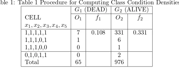
Table 1: Table 1 Procedure for Computing Class Condition Densities

the decision surface is defined by the equationg(x_{) = 0. The decision surface separates}

points assigned to w1 from points assigned tow2. The decision surface is a hyperplane wheng(x_{) is linear.}

If x_{1 and} x_{2 are both on the decision surface, then} wT_x

1 +w0 = wTx2 +w0 or

wT_(x

1−x2) = 0 [1]

w _{is normal to any vector that lies in the hyperplane. The feature space is divided}

by the hyperplane into two half-spaces: decision regionR1 forw1 and regionR2 forw2. Sinceg(x_{)>0 if} x_{is inR1, it follows that the normal vector}w _{points intoR1.}

3

Material and Methods

3.1

Material

To show the computation of discrete discriminant model, the secondary data of safe-motherhood collected by [5] that include group assignment (mother : dead, alive), five discriminator variables (x) such as place of delivery baby (x1), person who delivered baby (x2), antenatal care (x3), place of antenatal care (x4), and referal services obtained (x5). The total number of subjects to be analyzed is 1041 persons, among them 65 persons were dead and 976 persons were alive.

3.2

Methods

The class condition densities in G1 and G2 are computed by formula as follows: ˆfi(x) = ni(x)

The discrimination score inG1 and G2 are computed by formula as follows: ˆgi(x) = ni For demonstrating three other statistical analysis, the data were analyzed by means of statistical soft-ware such as SPSS and S-Plus.

4

(Results and Discussion

4.1

Discrete Discriminant Analysis

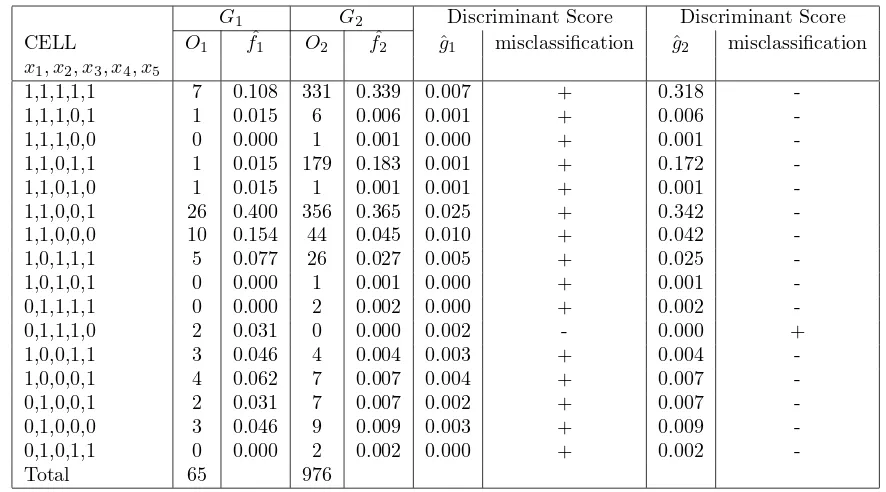
Table 2: Table 2 Discriminant Scores and Misclassification

G1 G2 Discriminant Score Discriminant Score CELL O1 f1ˆ O2 f2ˆ ˆg1 misclassification g2ˆ misclassification

x1, x2, x3, x4, x5

1,1,1,1,1 7 0.108 331 0.339 0.007 + 0.318 -1,1,1,0,1 1 0.015 6 0.006 0.001 + 0.006 -1,1,1,0,0 0 0.000 1 0.001 0.000 + 0.001 -1,1,0,1,1 1 0.015 179 0.183 0.001 + 0.172 -1,1,0,1,0 1 0.015 1 0.001 0.001 + 0.001 -1,1,0,0,1 26 0.400 356 0.365 0.025 + 0.342 -1,1,0,0,0 10 0.154 44 0.045 0.010 + 0.042 -1,0,1,1,1 5 0.077 26 0.027 0.005 + 0.025 -1,0,1,0,1 0 0.000 1 0.001 0.000 + 0.001 -0,1,1,1,1 0 0.000 2 0.002 0.000 + 0.002 -0,1,1,1,0 2 0.031 0 0.000 0.002 - 0.000 + 1,0,0,1,1 3 0.046 4 0.004 0.003 + 0.004 -1,0,0,0,1 4 0.062 7 0.007 0.004 + 0.007 -0,1,0,0,1 2 0.031 7 0.007 0.002 + 0.007 -0,1,0,0,0 3 0.046 9 0.009 0.003 + 0.009 -0,1,0,1,1 0 0.000 2 0.002 0.000 + 0.002 -Total 65 976

Table 3: Table 3 Degree of Misclassification Using Linear Discriminant Analysis Prediction Group Membership

Original Group Membership G1 (Dead) G2 (Alive) Total

G1 (Dead) 30 35 65

G2 (Alive) 104 872 976 Total 134 907 1041

The degree of misclassification is (63+0)/1041 = 6.05

Hence, the degree of correct classification is (2+976)₁₀₄₁ = 93.95%

4.2

Linear Discriminant Analysis

The degree of misclassification is (35+104)₁₀₄₁ = 13.4% The degree of correct classification is 86.6

4.3

Logistic Regression Analysis

The degree of misclassification is ₁₀₄₁(65) = 6.24% The degree of correct classification is 93.76

4.4

Neural Network Analysis

The degree of misclassification is ₁₀₄₁(65) = 6.24% The degree of correct classification is 93.76

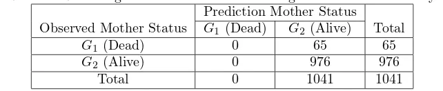
Table 4: Table 4 Degree of Misclassification Using Logistic Regression Analysis Prediction Mother Status

Observed Mother Status G1 (Dead) G2 (Alive) Total

G1(Dead) 0 65 65

Table 5: Table 5 Degree of Misclassification Using Neural Network Analysis Prediction Mother Status

Observed Mother Status G1(Dead) G2 (Alive) Total

G1 (Dead) 0 65 65

G2 (Alive) 0 976 976 Total 0 1041 1041

The first method gives the highest degree of correct classification. However, it is time consumed to compute for researchers who are not familiary with mathematical compu-tation. For those who understand the program language such as Fortran, S-plus etc., they can develop statistical software so that it can reduce time operation as well as the well-known statistical software. The second method gives the lowest degree of correct clas-sification. The third and fourth methods gives the same degree of correct clasclas-sification. However, the fourth method requires the understanding about program language such as S- Plus. The third method is preferred by researchers who are familiary with statistical software such SPSS, SAS, MINITAB.

5

Conclusion and Recommendation

Discrete discriminant analysis gives 93.95% correct classification, while linear discriminant analysis, logistic regression analysis, and neural network discriminant analysis give respec-tively 86.6Discrete discriminant analysis seems to be the most effective in discriminating individuals into groups when the discriminator variables are dichotomously categorical.

Discrete discriminant analysis is recommended for researchers who feel convenient in doing mathematical calculation using spreadsheet software. However, for those who prefer easy statistical software, logistic regression is recommended.

References

[1] ¨Omer Cengiz C¸ ELEB´I http://www.celebisoftware.com/Tutorials/neural networks/ accessed in 30 June 2009 at 7.50pm. Celebisoftware (2009)

[2] W.R. Dillon and M. Goldstein,Multivariate Analysis Methods and Applications, John Wiley and Sons, Inc., New York (1984).

[3] D.G. Kleinbaum , L.L. Kupper and K.E. Muller, Applied Regression Analysis and Other Multivariable Methods, PWS-Kent Publishing Company, Boston (1988). [4] D.G. Kleinbaum , L.L. Kupper, K.E. Muller and A.NizamApplied Regression Analysis

and Other Multivariable Methods, Duxbury Press, Pacific Grove (1998).