1257 Journal Homepage: -www.journalijar.com
Article DOI:
Article DOI:10.21474/IJAR01/1325 DOI URL: http://dx.doi.org/10.21474/IJAR01/1325
RESEARCH ARTICLE
COMPLEXITY ANALYSIS OF REORDERING ALGORITHMS FOR THE IMPLEMENTATION OF MULTIFRONTAL SOLUTION TECHNIQUE.
Anchu C.
Post Graduate student, Government Engineering College, Idukki, Kerala, India.
………
....
Manuscript Info
Abstract
……….
………
Manuscript History
Received: 12 June 2016 Final Accepted: 22 July2016 Published: August 2016
Key words:-
Solution of large order sparse system of equations need to be optimized on numerical computers in terms of memory usage and execution time. This optimization includes rearranging the equations in terms of its position and identifying submatric blocks where dense matrix operations can be defined.Direct solution methods of linear system of equation are based on factorization of coefficient matrix to set the solution. This thesis studies the effect of cholesky factorization of symmetric sparse matrices for reducing fill-ins and factorization
time. The study is carried out on ISRO’s in-house developed finite element structural analysis software, FEASTSMT direct solution schemes. The reordering techniques used here are Approximate minimum degree ordering (AMD), Column approximate minimum degree ordering (COLAMD), Multiple minimum degree ordering (MMD) and METIS. Since the finite element models of launch vehicle and satellite structures result in vary large order sparse system of equations, a variation of cholesky method called multifrontal scheme based on element connectivity information is used. The studies were carried out on basic large order 1D, 2D , 3D models as well as the models involving combination of these three types. Complexity of these algorithms depends on the data structure of assembly tree, which is a relationship between submatrices. The overall execution time , average, worst and best case time complexities of the multifrontal method with respect to number of partial factorization were studied and presented in this thesis.
Copy Right, IJAR, 2016,. All rights reserved.
………
....
Introduction:-
FEAST (Finite Element Analysis of Structures) is ISRO's structural analysis software based on Finite Element Method (FEM) realized by Structural Engineering Entity of Vikram Sarabhai Space Centre (VSSC). Substructured and Multi-Threaded (SMT) implementation of the solver ensures high performance of the software to the end users. Numerical computational aspects are the core of FEASTSMT.PreWin is the graphical user interface based pre and post processor, developed using state of the art graphical processing technology. FEASTSMT is a FE solver module, built as dynamic link library (DLL), integrated with pre and post processor as shown in Fig.1.
Corresponding Author:-Anchu C
1258 Fig.1:- Architecture model of PreWin/FEASTSMT.
The system of linear equations arising from a linear solution of a structure with n degree of freedoms is written as: }
{ } ]{
[K d f (1)
whereKis the n by n stiffness matrix, fis a vector of size n, which stores the loading at each degree of freedom (dof), and dis a vector of size n, which stores the unknown displacement corresponding to the loading.
There are two main classes of methods for the solution of sparse linear systems: direct methods, that are based on a factorization of A (e.g., LU or QR), and iterative methods, that build a sequence of iterates that hopefully converges to the solution. Direct methods are acknowledged for their numerical stability but often have large memory and computational requirements, while iterative methods are less memory demanding and often faster but less robust in general; the choice of a method is usually complicated since it depends on many parameters such as the properties of the matrix and the application.
The various numerical aspects of FEASTSMT are included in 1. Here sparse system of equations are considered. Cholesky factorization is used for those models having smaller dimension but results in larger number of fill-ins. So the main task is to reduce the number of fill-ins.
Reordering algorithms can be used for reducing the amount of fill-in by rearranging the initial matrix according to the generated permutation order. The various minimum degree reordering algorithms were defined in detail in 2. Here the analysis is carried out on approximate minimum degree ordering 3, column approximate minimum degree ordering 4,Multiple Minimum Degree ordering 5 and METIS 6. Here each routine returns a permutation vector P of size n, where P[k] = i if row and column i are the kth row and column in the permuted matrix . This permuted vector can be used for reordering the matrix and thereby reducing the amount of fill-in.
Cholesky solution method for interface variables requires global stiffness matrix to be assembled. This creates memory related issues for large order problems and cannot exploit parallel processing system architectures to reduce overall solution time. Since sparse storage schemes are employed to reduce active memory requirements, dense matrix operations, which uses system cache memory are not implemented in the SMT solver for matrix algebra, which is given as detailed in 7.
Multifrontal method is included in detail in section 2 ,which mainly includes both forward elimination and backward substitution algorithms and the assembly tree construction process. Section 3 mainly focuses on the various reordering routines and their advantages and later in section 4, which includes some test problems and their results are concluded.
Multifrontalmethod:-
1259 partially assembled dofs. Typically, we exploit the supernodes and there are multiple dofs eliminated at a frontal matrix.Therefore, we can use a blocked form of the partial factorization that can be written as
matrices Bnexne,Vnrxne and Cnrxnr where ne and nr are the number of eliminated and remaining dofs respectively. Bis a square matrix corresponding to the eliminated degrees of freedom’s (dof), Cis a square matrix corresponding to the remaining dofs, and Vis a rectangular matrix which couples the eliminated and remaining dofs. After the partial factorization is completed, Bstores the diagonal factors LB, Vstores the off-diagonal factors and Cstores the
Schurcomplement .
Once the factors are calculated, the triangular solution can be performed by forward elimination and back substitution. The forward elimination for an assembly tree node can start as soon as the factors corresponding to fully assembled dofs are computed. Alternatively, the factorization and forward elimination can be separated by starting the forward elimination after all factorization steps are completed. The back substitution, on the other hand, must wait until all forward elimination tasks are completed.
Forward Elimination:-
The forward elimination , involves solving Ly = b for y.Frontal RHS matrices are used to perform forward eliminationand back substitution operations efficiently on dense matrix blocks. In addition to the frontal matricesthat stores the factors for the eliminated dofs, RHS frontal matrices stores the loads and partial results for the eliminated and remaining dofs. For the forwardelimination steps, the frontal matrix and loads on the corresponding dofs are written in ablocked form as follows:
Where Fe and Fr store the loads updated with the partial solution on the eliminatedand remaining dofs respectively.
The right-hand side matrix in Equation (3) is referred to as RHSfrontal matrix. When the forward elimination steps are complete, Fe stores Ye, the resultsof the forward elimination for the fully assembled dofs. Fr, on the other hand,
stores Yr,the contribution from the current assembly tree node to the forward elimination steps atthe parent assembly
tree node.
For forward elimination, the dense matrix operationson the frontal matrix are given as follows:
F
whereYe is the results from the forward elimination and
F
u
r is the contributionfrom the currently processed tree node to the forward elimination steps at the parent tree node.
Backward Substitution:-
The backward substitution, consisting in solving Ux = y for x. After forward elimination is finished, the solution iscompleted by a backsubstitution. For the back substitution steps, the frontal matrix and RHS vectors can bewritten in the blocked matrix form as follows:
thecurrent frontal matrix determines De. The entries of Ye are the values computed in theforward elimination phase
from Equation (4). Dr stores the displacements for theremainingdofs, which are found at an ancestor of the current
(3)
(4)
(5)
1260 tree node. XandYrarenotused for the back substitution operations on the frontal matrix. Matrix operations for the
back substitution are given as:
D
L
Y
Y
rT off e u
e
Y
L
D
ueT B
e
After the displacement matrix De is computed, it isdisassembled to Drmatrices of the children elements.
Fig.2:- Direction of the dependencies between the factorization and triangular solution tasks for an assembly tree data structure.
A partial factorization is performed for each frontal matrix corresponding to an assembly tree node. The dependencies between the partial factorization tasks are shown in Fig.2 for an example assembly tree. For the factorization, the tree nodes are visited in a postorder tree traversal, for which the children of an assembly tree node are visited before the parent node. A single active frontal matrix is used for the numerical factorization for the serial factorization. For multithreaded factorization, the active frontal matrices are as many as the number of threads used for the factorization if the tree-level parallelism is exploited.
Assembly tree:-
The assembly tree represents the dependency between the partial factorization tasks 1. A parent node in the assembly tree can only be processed after all of its children are assembled to the corresponding frontal matrix. Leaf nodes of the assembly tree represent the finite elements, whereas, the internal nodes represent the intermediate elements obtained by the assembly and condensation of the children nodes. Once all children of an intermediate node are processed, its stiffness matrix can be assembled and fully summed DOFs of the element can be condensed.
Fig.3illustrates the assembly tree using a 4×4 mesh.The gray nodes represent the finite elements in the model. There are four subtrees processed by different threads. Here, FE’s are shown in gray color and they are not considered as
assembly tree nodes. The FE’s are stored at the leaves of the assembly tree. The black nodes shown in Fig.3 are assemblytree nodes for a nested dissection matrix ordering.
Fig.3:- Assembly tree structure for the example 4×4 mesh.
1261
Reordering algorithms:-
The reordering algorithms considered for analysis includes minimum degree algorithms and multilevel k-way partitioning algorithms. The minimum degree idea aims to minimize fill locally at each step of the elimination game by choosing to eliminate a vertex with the minimum degree in theelimination graph. The minimum degree algorithms considered here for analysis includes Approximate Minimum Degree ordering(AMD), Column Approximate Minimum degree ordering (COLAMD)and Multiple minimum Degree ordering(MMD).Similarly METIS is used for the multilevel partitioning of the graph and thereby minimizes the fill-ins encountered during factorization process. Each of this algorithms computes a permutation order and reorders the input sparse matrix according to the permutation order. Reordering not only reduces the amount of fill-ins but also reduces the number of computations.
Approximate Minimum Degree ordering:-
AMD is a set of routines for preordering a sparse matrix prior to numerical factorization. It uses an approximate minimum degree ordering algorithm 3 to find a permutation matrix P and the reordered matrix after factorization has fewer nonzero entries than the original matrix .
In a graph G, two adjacent vertices u and v are said to be indistinguishable ifadj(u) U adj(u) = adj(v) U adj(v). Clearly, if u and v are indistinguishable then they havethe same degree, and if one of them, say u, is eliminated, no new fill edges joiningv to any other neighbor of u are created. The degree of v will decrease by onein the remaining graph. Thus if one of them is amongthe vertices with minimum degree, then they both are, and after the elimination ofone, the other will continue to be among the vertices with minimum degree in thenext elimination graph. For this reason, both vertices could be eliminated at thesame step, and numbered consecutively in a minimum degree ordering. Two vertices that become indistinguishable at one step of theelimination game remain indistinguishable for the rest of the algorithm. In addition,they can be eliminated together whenever one of them is chosen for elimination . Thus for purposes of the MD algorithm, the two vertices can be merged into a supernode and treated as one vertex for the remainder of the algorithm. This is called mass elimination in MD implementations. The major limitation of using MD algorithm is the calculation of exact degrees of vertices. For this reason variants of minimum degree algorithms were implemented and AMD is one of them, which is based on approximate degree calculation of each vertex according to some heuristics.
The most costly part of the minimum degree algorithm is the recomputation of the degrees of nodes adjacent to the current pivot element. Rather than keep track of the exact degree, the approximate minimum degree algorithm finds an upper bound on the degree that is easier to compute. For nodes of least degree, this bound tends to be tight. Like MD, and unlike MMD, the Approximate Minimum Degree (AMD) algorithmis a single elimination algorithm; hence the degree and graph updates are performedafter a single supernode is eliminated.Using the approximate degree instead of the exact degree leads to a substantial savings in run time, particularly for very irregularly structured matrices. It has no effect on the quality of the ordering.
Column Approximate Minimum Degree ordering:-
Column approximate minimum degree ordering (COLAMD) method is based on the symbolic LU factorization algorithm. At step k, we select a pivot column c to minimize some metric on all of the candidate pivot columns as an attempt to reduce fill-in. Columns c and k are then exchanged. The choice of pivot column c is a heuristic. The presence of dense (or nearly dense) rows or columns in A can greatly affect both the ordering quality and run time.
Taking advantage of supercolumns can greatly reduce theordering time. In the symbolic update step, all columns j in the set Rranalysed. If any two or more columns have the same pattern (tested via a hash function 4 ), they are
merged into a single super-column. This saves both time and storage in subsequent steps. Selecting a super-column c allows us to mass-eliminate all columns [c] represented by the super-column c, and we skip ahead to step k + |[c]| of symbolic factorization.
Multiple Minimum Degree ordering:-
1262 this case, eliminating the snodes of K before other snodes of possibly lower degree will generate a slightly perturbed minimum degree ordering. However, in practice the quality of the orderings from the MMD algorithm is usually even better than orderings from the MD algorithm with respect to fill.
METIS:-
Graph partitioning algorithms are also used to compute fill-reducing orderings of sparse matrices. These fill reducing orderings are useful when direct methods are used to solve sparse systems of linear equations. A good ordering of a sparse matrix dramatically reduces both the amount of memory as well as the time required to solve the system of equations. Furthermore, the fill-reducing orderings produced by graph partitioning algorithms are particularly suited for parallel direct factorization as they lead to high degree of concurrency during the factorization phase.
The algorithms implemented in METIS are based on the multilevel graph partitioning paradigm 6. The multilevel paradigm, illustrated in 6, consists of three phases: graph coarsening, initial partitioning, and uncoarsening. In the graph coarsening phase, a series of successively smaller graphs is derived from the input graph. In the initial partitioning phase, a partitioning of the coarsest and hence, smallest, graph is computed using relatively simple approaches such as the algorithm developed by Kernighan-Lin 6.The three phases of multilevel k-way partitioning is shown in Fig.4. Since the coarsest graph is usually very small, this step is very fast. Finally, in the uncoarsening phase, the partitioning of the smallest graph is projected to the successively larger graphs by assigning the pairs of vertices that were collapsed together to the same partition. Because of the presence of graph partitioning METIS provides much more improved results than other reordering methods , especially for three dimensional models of large number of nodes.
Fig.4:- Three phases of multilevel k-way partitioning. Test Problems:-
This section contains the various test problems as well as the results including the time for factorization and amount of fill-ins occurred after factorization .
1263 Properties of Model 1:-
Nodes 3244
2D Elements 2686
Degrees of freedom 16206
Matrix size 52572264x52572264
Fig.6:- Model 2.
Properties of Model 2:-
Nodes 3875
2D Elements 2778
Degrees of freedom 17220
Matrix size 3606916x3606916
Fig.7:- Model 3.
Properties of Model 3:-
Nodes 5616
3D Elements 4000
Degrees of freedom 15768
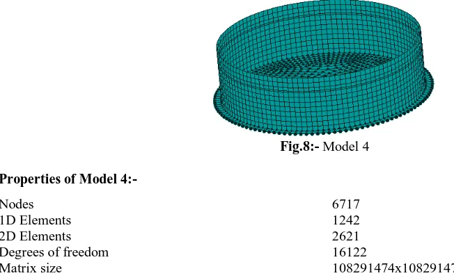
1264 Fig.8:- Model 4
Properties of Model 4:-
Corresponding to each model the amount of fill-in and cholesky factorization time is given in
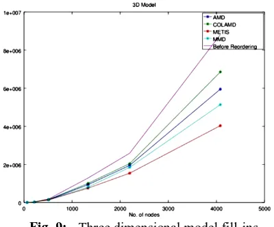
Table 1. Fill-ins in model 2 is very large compared to other three models this is because of its larger degrees of freedom which leads to biggermatrices. For all four models fill-ins before reordering is very high and the various reordering algorithm is then applied to reduce this fill-in. It is found that METIS generated better results compared to other three methods if the model size is increased. Similarly factorization timeis also analyzed and it shows that cholesky factorization takes more time for its computation and is not suitable for those models which are larger in size.
Table 1:-Cholesky factorization time and fill-in.
For three dimensional models of increasing size the effect of various reordering techniques are shown in Fig .9.
Nodes 6717
1D Elements 2D Elements
1242 2621
Degrees of freedom 16122
Matrix size 108291474x108291474
MODEL Fill-ins Before reordering
Reordering Routine
Fill-in Fact. Time
AMD COLAMD MMD METIS
Fill-in Fact.
Time Fill-in
Fact. Time
Fill-in Fact. Time
1265 Fig .9:- Three dimensional model fill-ins.
Due to the limitations of cholesky factorization method ,multifrontal method with multithreading feature is used. The factorization time in multifrontal method is shown inTable 2.
Table 2:-Multifrontal solution time
The factorization time using multifrontal method is more effective than cholesky factorization. This is because of its multithreading feature in assembly tree levels. Therefore multifrontal method can be used for solving models of larger dimension.
Conclusion:-
In this thesis the various matrix reordering algorithms, their time and space complexity, multifrontal based direct solution schemes for large order linear systems were studied. The reordering algorithms includes Approximate Minimum Degree ordering (AMD), Column AMD (COLAMD), Multiple Minimum Degree ordering (MMD) and METIS. These reordering algorithms generates a permutation order for the algebraic system of equations formed based on engineering parameters. The reordering algorithm which is best suited for numerical model of practical launch vehicle structure is identified based on its complexity analysis. For one dimensional models of smaller number of nodes it is analysed that AMD is more suitable, Column AMD is more suitable for smaller two dimensional models and MMD is the best for three dimensional models of smaller sizes. But in the case of models of larger sizes ie. For 1D, 2D, 3D and also for those models having all these types of elements METIS is found to be best routine for FEASTSMT. This is because of the proper partitioning of graph structure. It is concluded that METIS reduces amount of fill-ins as well as the time required for factorization. In the case of cholesky factorization the amount of time required for partial factorization increases with respect to the model size but in the case of multifrontal method due to the presence of multithreading feature it considerably reduces the amount of time for factorization. Thus METIS routine along with multifrontal method reduces the memory requirement as well as the overall execution time for factorization.
Acknowledgment:-
The authors duly acknowledge the help rendered by Shri. DEEPAK P,Scientist/Engineer ‘SE’, SMSD/SDMG/STR, VSSC, ISRO,Thiruvananthapuram , in understanding reordering algorithms for the implementation of multifrontal solution technique.
References:-
1. High-performance direct solution Of finite element problems on Multi-core processors: Murat EfeGuney 2. An Object_Oriented Collection of Minimum Degree Algorithms Design_ implementation_ and Experiences:
Gary Kumfert, Alex Pothen
MODEL Reordering Routine(Time in sec)
AMD COLAMD MMD METIS
Model 1 6 8 7 6
Model 2 11 10 8 7
Model 3 8 26 9 8
1266
3. P. R. Amestoy, T. A. Davis, and I. S. Du_. An approximate minimum degree ordering algo-rithm. SIAM J. Matrix Anal. Applic., 17(4):886{905, 1996}.
4. T. A. Davis, J. R. Gilbert, S. I. Larimore, and E. G. Ng. A column approximate minimum degree ordering algorithm. ACM Trans. Math. Softw., 30:353{376, 2004.
5. The Computational Complexity of the Minimum Degree Algorithm: P. Heggernes, S. C. Eisenstat, G. Kumfert, A. Pothen.
6. A Software Package for Partitioning Unstructured Graphs, Partitioning Meshes, and computing Fill-Reducing Orderings of Sparse Matrices: George Karypis, Vipin Kumar.