Multiplicative Updates for Non-negative
Projections
Zhirong Yang
a,∗
, Jorma Laaksonen
aaLaboratory of Computer and Information Science,
Helsinki University of Technology, P.O. Box 5400, FI-02015 HUT, Espoo, Finland
Abstract
We present here how to construct multiplicative update rules for non-negative pro-jections based on Oja’s iterative learning rule. Our method integrates the multi-plicative normalization factor into the original additive update rule as an additional term which generally has a roughly opposite direction. As a consequence, the modi-fied additive learning rule can easily be converted to its multiplicative version, which maintains the non-negativity after each iteration. The derivation of our approach provides a sound interpretation of learning non-negative projection matrices based on iterative multiplicative updates—a kind of Hebbian learning with normalization. A convergence analysis is scratched by interpretating the multiplicative updates as a special case of natural gradient learning. We also demonstrate two application examples of the proposed technique, a non-negative variant of the linear Hebbian networks and a non-negative Fisher Discriminant Analysis, including its kernel ex-tension. The resulting example algorithms demonstrate interesting properties for data analysis tasks in experiments performed on facial images.
Key words: Non-negative projection; Multiplicative update; Oja’s rule; Hebbian learning; Matrix factorization
1 Introduction
Projecting high-dimensional input data into a lower-dimensional subspace is a fundamental research topic in signal processing and pattern recognition. Non-negative projection is desired in many real-world applications, for example, for
∗ Corresponding author.
Email addresses: [email protected] (Zhirong Yang),
images, spectra etc., where the original data are non-negative. However, most classical subspace approaches such as Principle Component Analysis (PCA) andFisher Discriminant Analysis (FDA), which are solved bySingular Value Decomposition (SVD), fail to produce the non-negativity property.
Recently, Lee and Seung [12,13] introduced iterative multiplicative updates, which are based on the decomposition of the gradient of given objective func-tion, for non-negative optimizations. They applied the technique to the Non-negative Matrix Factorization (NMF) which seems to yield sparse represen-tations. Several variants of NMF such as [5,22,24] have later been proposed, where the original NMF objective function is combined with various regular-ization terms. More recently, Yuan and Oja [23] presented a method called
Projective Non-negative Matrix Factorization (P-NMF) without any addi-tional terms, but directly derived from the objective function of PCA net-works except that the projection was constrained to be non-negative. The simulation results of P-NMF indicate that it can learn highly localized and non-overlapped part-based basis vectors. However, none of the above works provides an explanation why the multiplicative updates can produce sparser and more localized base components.
The multiplicative update rules of the above algorithms are based on decom-position of the gradients of an objective function into positive and negative parts, one as the numerator and the other as the denominator. Nevertheless, such method would fail when the gradient is not naturally expressed in posi-tive and negaposi-tive parts. Sha et al. [21] proposed an alternaposi-tive decomposition of the gradient and applied it to the minimization of a quadratic objective. This method albeit cannot handle the situation where the gradient contains only one positive (negative) term. Furthermore, how to combine orthogonality or quadratic unit norm constraints with this method is still unknown.
In this paper we present a more general technique to reformulate a variety of existing additive learning algorithms to their multiplicative versions in order to produce non-negative projections. The derivation is based on Oja’s rule [17] which integrates the normalization factor into the additive update rule. Therefore, our method provides a natural way to form the numerator and denominator in the multiplicative update rule even if external knowledge of gradient decomposition is not available. Another major contribution of our approach is that its derivation also provides a sound interpretation of the non-negative learning based on iterative multiplicative updates—a kind of Hebbian learning with normalization.
interpre-tation why P-NMF can learn non-overlapped and localized basis vectors. In the supervised FDA learning, our non-negative variant of theLinear Discrim-inant Analysis (LDA) can serve as a feature selector and its kernel extension can reveal an underlying factor in the data and be used as a sample selector. The resulting algorithms of the above examples are verified by experiments on facial image analysis with favorable results.
The remaining of the paper is organized as follows. First we introduce the basic idea of multiplicative update rules in Section 2. The non-negative projection problem is then formulated in Section 3. In Section 4 we review Oja’s rule and present the technique how to use it in forming the multiplicative update rules. The proposed method is applied in two examples in Section 5: one for unsupervised learning and the other for supervised. The experimental results of the resulting algorithms are presented in Section 6. Finally, conclusions are drawn in Section 7.
2 Multiplicative Updates
Suppose there is an algorithm which seeks an m-dimensional solution wthat maximizes an objective functionJ(w). The conventionaladditive update rule for such a problem is
˜
w=w+γg(w), (1) where ˜w is the new value of w, γ a positive learning rate and the function
g(w) outputs an m-dimensional vector which represents the learning direc-tion, obtained e.g. from the gradient of the objective function. For notational brevity, we only discuss the learning for vectors in this section, but it is easy to generalize the results to the matrix case, where we will use capital letters
W and G.
The multiplicative update technique first generalizes the common learning rate to different ones for individual dimensions:
˜
w=w+ diag(η)g(w), (2)
whereηis anm-dimensional positive vector. Choosing different learning rates
for individual dimensions changes the update direction and hence this method differs from the conventional steepest-gradient approaches in the full real-valued domain.
It has been shown that the following choice of η has particular interesting
one can always choose ηi =wi/gi−, i= 1, . . . , m, such that the components of
The above multiplicative update maintains the non-negativity of w. In addi-tion,wi increases wheng+i > gi−, i.e. [g(w)]i >0, and decreases if [g(w)]i <0.
Thus the multiplicative change ofwi indicates how much the direction of that
axis conforms to the learning direction. There exists two kinds of stationary points in the iterative use of the multiplicative update rule (3): one satis-fies g+i = g−
i , i.e. g(w) = 0, which is the same condition for local optima
as in the additive updates (1), and the other is wi → 0. The latter
condi-tion distinguishes the non-negative optimizacondi-tion from convencondi-tional ones and yields sparsity inw, which is desired in many applications. Furthermore, un-like steepest gradient or exponential gradient [10], the multiplicative update rule (3) does not require any user-specified learning rates, which facilitates its application.
In most non-negative algorithms that use multiplicative updates (e.g. [13,21,24]), the convergence of the objective has been proven via an auxiliary function. However, such a function depends on particular update rules and sometimes could be difficult to find. Here we present a novel interpretation of multi-plicative updates as an optimization using natural gradient [1], which greatly simplifies the convergence analysis of the objective. Define the matrix G(w) as
[G(w)]ij =δij
g−i
wi
, (4)
withδij the Kronecker delta. The tensorGdefines a Riemannian inner product
hdw, dwiw=
Since G(w) is diagonal, its inverse can be computed by
h
Henceforth we can obtain the natural gradient ascend update [1] for w:
˜
a Riemannian manifold [1], the multiplicative updates form a steepest gradi-ent ascend method in (0,+∞)m which is curved by the tangent of the given
objective function. Therefore, the multiplicative update rule (3) guarantees monotonic increase of the objective function if ζ = 1 corresponds to a suffi-ciently small learning step and thus (7) forms a good approximation of the continuous flow in the Riemannian space.
3 Non-negative Projection
Subspace projection methods are widely used in signal processing and pattern recognition. An r-dimensional subspace out of ℜm can be represented by an
m×rorthogonal matrix W. In many applications one can write the objective function for selecting the projection matrix in the form
maximize
W J(W) =
1 2E
n
F kWTvk2o, (8)
where v is an input vector, F a function from ℜ to ℜ, and E{·} denotes the expectation. For problems whereF(x) =x, the objective (8) can be simplified to
maximize
W J(W) =
1 2Tr
WTEnvvToW. (9)
Such form covers the objectives of many classical analysis methods such as
Principal Component Analysis (PCA) and Fisher’sLinear Discriminant Anal-ysis (LDA). The motivation and neural architecture of (9) is justified in [11]. By setting A=EnvvTo, we can write the gradient of (9) as
∂J(W) ∂W =E
n
vvToW =AW. (10)
ObviouslyA is a positive semi-definite matrix.
The function F can be other than F(x) =x. For example, in [8] the log like-lihood function F(x) = logp(x) was used and a variant of Independent Com-ponent Analysis (ICA) was derived. In that case, A=EnF′kWTvk2vvTo
is a negative semi-definite matrix.
In summary, we consider a particular set of additive update rules with the learning direction G(W) = AW, where A is an m×m symmetric matrix.
4 Oja’s Rule in Learning Non-negative Projections
The multiplicative update rule described in Section 2 maintains the non-negativity. However, the gradient of projection objective yields a single term and does not provide any natural way to obtaing+ and g− (or G+ andG−). In this section we present a very simple approach to include an additional term for constructing the multiplicative update rules if the solution is constrained to be of unitL2-norm or orthogonal.
First let us look at the projection on a one-dimensional subspace. In many optimization problems the objective function J(w) is accompanied with the constraint
ω(w) =wTBw1/2 = 1, (11)
with B an m×m symmetric matrix. In particular, ω(w) = kwk if B =I. If
w is initialized to fulfill (11), the normalization step
wnew= ˜w(ω( ˜w))−1 (12)
maintains that the newwstill satisfies (11) sinceω(βw) = βω(w) for a scalar β.
One may try to combine the two update steps (1) and (12) into a single step version. The normalization factor (ω(w))−1 can be expressed using Taylor expansion as
(ω( ˜w))−1 =(w+γg)TB(w+γg)−1/2
=1 +γ(wTBg+gTBw) +O(γ2)−1/2
≈1− 1
2γ(w
TBg+gTBw). (13)
Hereg =g(w) for brevity and the final step is obtained by dropping all terms of O(γ2) or higher orders. Inserting this result and (1) into (12), we obtain
the following Oja’s single-step update rule [17]:
wnew≈w+1
2γ(2g−ww
TBg−wgTBw), (14)
where again the terms of O(γ2) have been dropped.
Now setting g(w) = Aw, we obtain a possible decomposition of g(w) into two non-negative parts as
where
0 otherwise. (16)
The simple update rule
winew =wi
usually yields poor results for non-negative projection problems. The situation is even more problematic whenA is non-negative, i.e. A−=0. As an alterna-tive, we here propose to substituteg from (15) into (14) and then obtain
wnew ≈w+1 2γ(2A
+w−2A−w−wwTBAw−wwTABw). (19)
Supposewis initialized with values in (0,1) and fulfills (11). All terms without their leading sign in the right side of (19) are then positive if wT(BA+
AB)w > 0 for all positive w. This condition defines the convexity of the solution subspace and is satisfied whenBA+ABis positive definite. Verifying such positive definity can easily be done before the iterative learning.
We can then apply the generalization technique described in Section 2 and obtain the following multiplicative update rule:
wnewi =wi
2 [A+w]i 2 [A−w]
i+ [wwT(BA+AB)w]i
. (20)
Since B is symmetric, (20) can be further simplified to:
winew=wi
[A+w]i [A−w]
i+ [wwTBAw]i
(21)
because in that case
wTBAw= (wTBAw)T =wTATBTw=wTABw. (22)
The original Oja’s rule for a single vector has been generalized to the matrix case [18]. It combines the following additive learning rule and normalization steps:
˜
W=W+γG(W) (23)
where W and Gare m×r matrices and
Ω(W) = I (25)
is the optimization constraint in the matrix case. IfΩ(W) = (WTW)1/2, the
normalization factor can be approximated by
Ω( ˜W)−1 ≈I− 1
2γ(W
TG+GTW), (26)
with similar derivation as in (13). Inserting (26) and (23) into (24), we obtain
Wnew≈W+ 1
2γ(2G−WW
TG−WGTW). (27)
By again applying the generalization onγ and insertingG=AW, we can get the following multiplicative update rule
Wijnew=Wij
[A+W]ij +hWWTA−Wi
ij
[A−W]
ij + [WWTA+W]ij
. (28)
Our method is suitable for problems with the constraint of the formWTW =I
orwTBw= 1, but generally it does not work for WTBW =Iif B 6=I. This is because such constraint ofB-uncorrelatedness is probably overwhelmed by the non-negative learning which tends to yield high orthogonality.
If one only considers the projection on the Stiefel manifold (i.e.WTW=I), a more straightforward derivation can be obtained by using the natural gradient. Given a learning direction G = AW, the natural gradient ascend update is [16]
Wnewnat =W+γG−WGTW. (29)
Substituting A = A+−A− and applying the reforming technique on γ, we obtain the same multiplicative update rule (28). This is not surprising because Oja’s rule and natural gradient are two essentially equivalent optimization methods on the Stiefel manifold except that the former is based on the ordinary Euclidean metric while the latter on a canonical Riemannian metric [4].
5 Examples
these examples is to demonstrate the applicability of the technique described in the previous section and to help readers get more insight in the reforming procedure.
5.1 Non-negative Linear Hebbian Networks
Using multiplicative updates for non-negative optimization stems from the
Non-negative Matrix Factorization (NMF) proposed by Lee and Seung [12]. Given an m ×n non-negative input matrix V where columns are the input samples, NMF seeks two non-negative matrices W and H which maximizes the following objective:
JN M F(W,H) = kV−WHkF. (30)
Herek · kF is the Frobenius matrix norm, defined as
kQkF =
X
ij
Q2ij (31)
for a matrixQ. The authors of [12] derived the following multiplicative update rules of NMF
Wijnew =Wij
h VHTi
ij
[WHHT] ij
, (32)
Hijnew =Hij
h
WTVi
ij
[WTWH] ij
. (33)
NMF is not as good as Principal Component Analysis (PCA) in minimizing the reconstruction error, but it was reported that NMF is able to extract some localized and part-based representations of the input samples [12]. To improve such localization effect, Yuan and Oja have recently developed a vari-ant of NMF called Projective Non-negative Matrix Factorization (P-NMF) [23], which is derived from the following optimization problem:
minimize
W≥0 JP-N M F(W) = kV−WW TVk
F. (34)
That is, P-NMF replaces the matrixH with WTV in the objective function. This change makes P-NMF also a variant of PCA whose objective is same as that of P-NMF except the non-negative constraint. The unconstrained gradi-ent of JP−N M F(W) is given by
∂JP-N M F(W)
∂Wij
=−2hVVTWi
ij +
h
WWTVVTWi
ij +
h
VVTWWTWi
ij,
upon which the authors of [23] obtained the following multiplicative update rule using the technique in Section 2:
Wijnew =Wij
2hVVTWi ij
[WWTVVTW]
ij + [VVTWWTW]ij
. (36)
Similar to NMF, P-NMF is not the best method to minimize the reconstruction error. Instead, it focuses in training orthogonal basis vectors. The simulation results in [23] showed that P-NMF is capable of extracting highly localized, sparse, and non-overlapped part-based features. However, there is little expla-nation about this phenomenon in [23].
In this example we employ the reforming technique of the previous section to derive a new multiplicative update rule, named Non-negative Linear Heb-bian Network (NLHN), for finding the non-negative projection. Given an m -dimensional non-negative input vector v, we define the learning direction by the simplest linear Hebbian learning rule, i.e. the product of the input and the output of a linear network:
G=v(WTv)T =vvTW. (37)
Inserting this to (28) with vvT = A = A+, we obtain the following update rule:
Wijnew=Wij
h
vvTWi
ij
[WWTvvTW] ij
. (38)
This result is tightly connected to the PCA approach because the correspond-ing additive update rule
Wnew =W+γ(vvTW−WWTvvTW) (39)
is a neural network implementation of PCA [18], which results in a set of eigen-vectors for the largest eigenvalues of En(v−E{v})(v−E{v})To. However,
these eigenvectors and the principal components of data found by PCA are not necessarily non-negative.
In addition to the on-line learning rule (38), we can also use its batch version
Wijnew =Wij
h
VVTWi
ij
[WWTVVTW] ij
, (40)
whereV is an m×n matrix, each column for one non-negative input sample.
We can see that NLHN bridges NMF and P-NMF. While the latter replacesH
as a slight variant of P-NMF. To see this, let us decompose (35) into two parts
∂JP-N M F(W)
∂Wij
=hG(1)i
ij +
h G(2)i
ij, (41)
whereG(1)=−VVTW+WWTVVTWandG(2) =−VVTW+VVTWWTW.
It has been shown that G(2) has little effect in learning the principal direc-tions [9]. Thus, by dropping G(2), we obtain the same multiplicative update rule as (40) based on G(1). Unlike other variants of NMF such as [5,14,22], NLHN does not require any additional regularization terms. This holds also for P-NMF.
The major novelty of NLHN does not lie in its performance as we have shown that it is essentially the same as P-NMF. We will also show by experiments in Section 6.2 that NLHN behaves very similarly to P-NMF. However, the inter-pretation of P-NMF as a variant of simple Hebbian learning with normaliza-tion helps us understand the underlying reason that P-NMF and NLHN are able to learn more localized and non-overlapped parts of the input samples.
As we know, iteratively applying the same Hebbian learning rule will result in that the winning neuron is repeatedly enhanced, and the normalization forces only one neuron to win all energy from the objective function [7]. In our case, this means that only one entry of each row ofW will finally remain non-zero and the others will be squeezed to zero. That is, the normalized Hebbian learning is the underlying cause of the implicit orthogonalization. Furthermore, notice that two non-negative vectors are orthogonal if and only if their non-zero parts are not overlapped.
Then why can P-NMF or NLHN produce localized representations? To see this, one should first notice that the objectives of P-NMF and NLHN are essentially the same ifWis orthonormal. Therefore, let us only consider here the objective of NLHN,JN LHN(W) =E
n
kWTvk2o, which can be interpreted as the mean
correlation between projected vectors. In many applications, e.g. facial images, the correlation often takes place in neighboring pixels or symmetric parts. That is why P-NMF or NLHN can extract the correlated facial parts such as lips and eye brows, etc.
We can further deduce the generative model of P-NMF or NLHN. Assume each observation v is composed of r non-overlapped parts, i.e. v = Pr
p=1vp.
In the context of orthogonality, P-NMF models each partvp by the scaling of
a basis vectorwp plus a noise vectorǫp:
vp =αpwp+ǫp. (42)
then the reconstructed vector of this part is
The norm of the reconstruction error is therefore bounded by
if 2-norm is used. Similar bounds can be derived for other types of norms. In words, wpwTpvp reconstructs vp well if the noise level ǫp is small enough.
According to this model, P-NMF or NLHN can potentially be applied to signal processing problems where the global signals can be divided into several parts and for each part the observations mainly distribute along a straight line modeled by αpwp. This is closely related to Oja’s PCA subspace rule[18],
which finds the direction of the largest variation, except that the straight line found by P-NMF or NLHN has to pass through the origin.
5.2 Non-negative Fisher Discriminant Analysis
Given a set of non-negative multivariate samples x(i), i = 1, . . . , n from the vector space ℜm, where the index of each sample is assigned to one of Q
classes,Fisher Linear Discriminant Analysis (LDA) finds the directionw for the following optimization problem:
maximize
Here SB is the between classes scatter matrix and SW is the within classes
scatter matrix, defined as:
SB =1
where nc and Ic are the number and indices of the samples in class c, and
µ(c)= 1
and hence becomes a particular case of (9).
The common solution of LDA is to attach the constraint (46) to the objective function with a Lagrange multiplier, and then solve the Karush-Kuhn-Tucker
multiplicative update technique described in Section 4 and obtain the follow-ing novel alternative method here named Non-negative Linear Discriminant Analysis (NLDA).
We start from the steepest-gradient learning:
g(w) = ∂(
1 2w
TS Bw)
∂w =SBw. (54)
Because both SB and SW are symmetric, we have A =SB and B= SW and (21) becomes
winew=wi
h S+Bwi
i
h S−Bwi
i+ [ww TS
WSBw]i
, (55)
with the elements ofwinitialized with random values from (0,1) andwTS Ww=
1 fulfilled. Here S+B and S−B are determined by (16). If the symmetric matrix
SWSB+ (SWSB)T =SWSB+SBSW is positive definite, then
wTSWSBw=
1 2
wTSWSBw+ (wTSWSBw)T
=1 2w
T(S
WSB+SBSW)w>0. (56)
That is, all terms on the right side of (55) are positive and so is the newwafter each iteration. Moreover, notice that NLDA does not require matrix inversion ofSW, an operation which is computationally expensive and possibly leads to
singular problems.
For a discriminant analysis of two classes C and ¯C, it is possible to improve the non-negative learning by preprocessing the data. For a dimension j, if median{xj|xj ∈C}>median{xj|xj ∈C¯}, we transform the original data by
xj ←Θj−xj, (57)
where Θj is the known upper bound of thej-th dimension. After such flipping,
for each dimensionj there exists a thresholdθj which is larger than more than
half of the samples ofC and smaller than more than half of the samples of ¯C. That is, the classCmainly distributes the inner part closer to the origin while
¯
C distributes the outer part farther from the origin. Projecting the samples to the direction obtained by (55) will thus yield better discrimination.
The above non-negative discriminant analysis can be extended to non-linear case by using the kernel technique. LetΦbe a mapping fromℜm toF, which
is implicitly defined by a kernel function k(x,y) = k(y,x) = Φ(x)TΦ(y).
the mapped space F, which is the solution of the optimization problem
maximize
w∈ℜm
1 2w
TSΦ
Bw (58)
subject to wTSΦTw= 1, (59)
whereSΦB andSΦW are the corresponding between-class and within-class scatter matrices. We use hereSΦ
T =S Φ B+S
Φ
W instead ofS Φ
W for simplification, but it is
easy to see that the problems are equivalent. From the theory of reproducing kernels [20] we know that any solution w ∈ F must lie in the span of all training samples inF. That is, there exists an expansion for w of the form
w=
n
X
i=1
αiΦ(x(i)). (60)
It has been shown [2] that by substituting (60) into (58) and (59), the uncon-strained KFDA can be expressed as
maximize α∈ℜn
1 2α
TKUK
α (61)
subject to αTKKα= 1, (62)
whereKij =k(x(i),x(j)),U= diag(U(1),U(2), . . . ,U(Q)), andU(j)is annj×nj
matrix whose elements are 1/nj.
The matricesKand Uare symmetric and all their elements are non-negative. We can obtain the following multiplicative update rule for novelNon-negative Kernel Fisher Discriminant Analysis (NKFDA) by setting A=A+ = KUK
and B=KKin (21):
αnewi =αi
[KUKα]i
[ααTKKKUKα]i. (63)
This formulation has the extra advantage that the resulting elements ofα
indi-cate the contribution of their respective samples in forming the discriminative projection. This is conducive to selecting among the samples and revealing the underlying factor in the data even if we only use the simple linear kernel, i.e. Φ(x) = x.
6 Experiments
Before proceeding to details, it should be emphasized that the goal of the non-negative version of a given algorithm usually differs from the original one. The resulting objective value of a non-negative algorithm generally is not as good as that of its unconstrained counterpart. However, readers should be aware of that data analysis is not restricted to reconstruction or classification and that non-negative learning can bring us novel insights in the data.
6.1 Data
We have used the FERET database of facial images [19]. After face segmen-tation, 2,409 frontal images (poses “fa” and “fb”) of 867 subjects were stored in the database for the experiments. We obtained the coordinates of the eyes from the ground truth data of FERET collection, with which we calibrated the head rotation so that all faces are upright. Afterwards, all face boxes were normalized to the size of 32×32, with fixed locations for the left eye (26,9) and the right eye (7,9). Each image were reshaped to a 1024-dimensional vector by column-wise concatenation.
Another database we used is the UND database (collection B) [6], which con-tains 33,247 frontal facial images. We applied the same preprocessing proce-dure to the UND images as to the FERET database.
6.2 Non-negative Linear Hebbian Networks
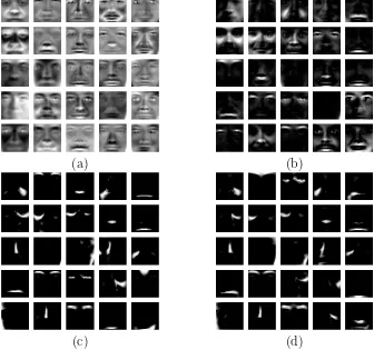
First we compared four unsupervised methods: PCA, NMF [12], P-NMF [23] and NLHN (40) for encoding the faces. The resulting basis images are shown in Figure 1. It can be seen that the PCA bases are holistic and it is hard to identify the parts that compose a face. NMF yields partially localized features of a face, but some of them are still heavily overlapped. P-NMF and NLHN are able to extract the highly sparse, local and non-overlapped parts of the face, for example the nose and the eyebrows. The major difference between P-NMF and NLHN is only the order of the basis vectors.
Orthogonality is of main interests for part-based learning methods because that property leads to non-overlapped parts and localized representations as discussed in Section 5.1. Suppose the normalized inner product between two basis vectors wi and wj is
Rij =
wTi wj
kwikkwjk
. (64)
(a) (b)
(c) (d)
Fig. 1. The top 25 learned bases of (a) PCA, (b) NMF, (c)P-NMF and (d) NLHN. All base images have been plotted without any extra scaling.
by the following ρ-measurement:
ρ= 1− P
i6=jRij
r(r−1) (65)
so that ρ ∈ [0,1]. Larger ρ’s indicate higher orthogonality and ρ reaches 1 when the columns ofW are completely orthogonal.
500 1000 1500 2000 2500 3000 3500 4000 4500 5000
Fig. 2.ρ values of NLHN, P-NMF and NMF with 25 basis vectors and
1024-dimen-sional data.
500 1000 1500 2000 2500 3000 3500 4000 4500 5000 0
500 1000 1500 2000 2500 3000 3500 4000 4500 5000 0
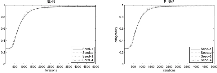
Fig. 3.ρ values of NLHN and P-NMF with different random seeds.
6.3 Non-negative Linear Discriminant Analysis
Next, we demonstrate the application of the linear supervised non-negative learning in discriminating whether the person in a given image has mustache and whether he or she is wearing glasses. The data was preprocessed by (57) before applying the NLDA algorithm (55). The positive definity requirement (56) was checked to be fulfilled for these two supervised learning problems.
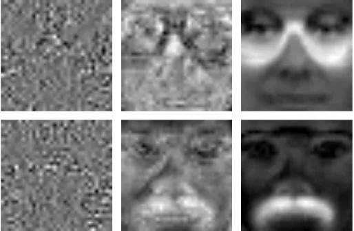
Fig. 4. Images of the projection vector for discriminating glasses (the first row) and mustache (the second row). The methods used from left to right are LDA, L-SVM, NLDA.
where C is a user-provided tradeoff parameter. By solving its dual problem
maximize α
n
X
i=1
αi−
1 2
n
X
i=1 n
X
j=1
αiαjy(i)y(j)x(i)x(j) (69)
subject to
n
X
i=1
αiy(i) = 0 and 0≤αi ≤C, i= 1,2, . . . , n, (70)
one obtains the optimalw=Pn
i=1αiy(i)x(i) with respect to the givenC.
Figure 4 displays the respective resulting LDA, L-SVM and NLDA projec-tion vectors as images. It is hard to tell from the LDA projecprojec-tion vector in which dimensions of the input samples are most relevant for discriminating mustache or glasses. Such poor filters are probably caused by overfitting be-cause LDA may require large amount of data to approximate the within-class covariance by SW but this becomes especially difficult for high-dimensional
problems. The filter images of L-SVM are slightly better than those of LDA. A distinguishing part can roughly be perceived between the eyes. Nevertheless there are still many irrelevant points found by L-SVM. In contrast, the NLDA training clearly extract the relevant parts, as shown by the brightest pixels in the rightmost images in Figure 4. Such results conform well to the human intuition in this task.
Table 1
Equal Error Rates (EERs) of training data (FERET) and test data (UND) in clas-sification of glasses versus no glasses.
LDA L-SVM NLDA
FERET 0.98% 11.69% 17.54%
UND 32.35% 25.23% 23.88%
L-SVM requires choice of the tradeoff parameter C. To our knowledge, there are no efficient and automatic methods for obtaining its optimal value. In this experiment we trained different L-SVMs with the tradeoff parameter in
{0.01,0.03,0.1,0.3,1,3,10,30,100} and it turned out that the one with 0.03 performed best in five-fold cross-validations. Using this value, we trained an L-SVM with all training data and ran the classification on the test data. The result shows that L-SVM generalizes better than LDA, but the test error rate is still much higher than the training one, which is possibly because of some overfitting dimensions in the L-SVM filter. Higher classification accuracy could be obtained by applying nonlinear kernels. This however requires more effort to choose among kernels and associated kernel parameters, which is beyond the scope of this paper.
The last column of Table 1 shows that NLDA performed even better than L-SVM in classifying the test samples. This is possibly because of the variation between the two databases. In such a case, the NLDA filter, which resembles more our prior knowledge, tends to be more reliable.
6.4 Non-negative Kernel Fisher Discriminant Analysis
Furthermore, we tested the function of NKFDA (63) that ranks the training samples by their contribution to the projection. We used only the linear kernel here because of its simplicity. After training of NKFDA on the FERET data labeled whether the subject has mustache, we sorted the training samples in the order of their respective values of αi.
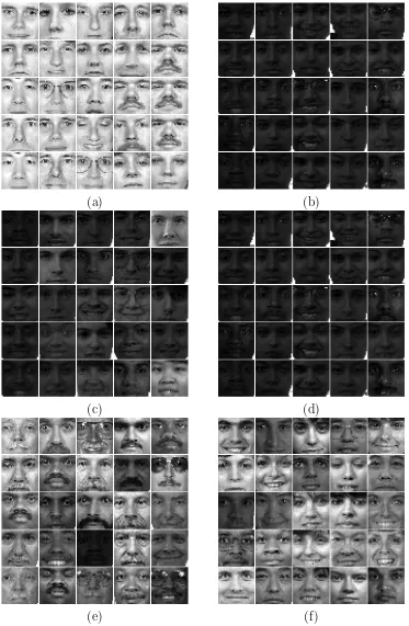
The top 25 faces and the bottom 25 faces are shown in Figures 5 (a) and (b), respectively. It can be clearly seen that the most important factor is the lighting condition. This could be expected because we are using well-aligned facial images of front-pose and neutral expression. Therefore the most significant noise here can be assumed to be variation in lighting. In addition, this order agrees with the common perception of humans, where the lighting that provides enough contrast helps in discriminating semantic classes.
(a) (b)
(c) (d)
(e) (f)
Fig. 5. The images with: (a) largest and (b) smallest values inαtrained by NKFDA;
(c) largest and (d) largest absolute values in α trained by KFDA; (e) largest and
Because the coefficients produced by KFDA are not necessarily non-negative, we sorted the faces by their absolute values. The bottom images look similar to those obtained by NKFDA. That is, darker images that provide poor contrast contribute least to the discrimination. However, it is hard to find a common condition or easy interpretation for the KFDA ranking of the top faces.
The resulting top and bottom facial images of L-SVM are shown in Figures 5 (e) and (f). As we know, the samples with non-zero coefficients are support vectors, i.e. those around the classification boundary, which explains the top images ranked by L-SVM. On the other hand, the samples far away from the boundary will be associated with zero coefficients. In this case, they are mostly typical non-mustache faces shown in Figure 5 (f).
7 Conclusions
We presented a technique how to construct multiplicative updates for learning non-negative projections based on Oja’s rule, including two examples of its ap-plication to reforming the conventional PCA and FDA to their non-negative variants. In the experiments on facial images, the non-negative projections learned by using the novel iterative update rules have demonstrated inter-esting properties for data analysis tasks in and beyond reconstruction and classification.
References
[1] S. Amari. Natural gradient works efficiently in learning. Neural Computation,
10(2):251–276, 1998.
[2] G. Baudat and F. Anouar. Generalized discriminant analysis using a kernel
approach. Neural Computation, 12(10):2385–2404, 2000.
[3] N. Cristianini and J. Shawe-Taylor. An Introduction to Support Vector
Machines. Cambridge University Press, 2000.
[4] A. Edelman. The geometry of algorithms with orthogonality constraints.SIAM
J. Matrix Anal. Appl., 20(2):303–353, 1998.
[5] T. Feng, S. Z. Li, H. Y. Shum, and H. J. Zhang. Local non-negative matrix
factorization as a visual representation. InProceedings. The 2nd International
Conference on Development and Learning, pages 178–183, 2002.
[6] P. J. Flynn, K. W. Bowyer, and P. J. Phillips. Assessment of time dependency
in face recognition: An initial study.Audio- and Video-Based Biometric Person
Authentication, pages 44–51, 2003.
[7] S. Haykin. Neural Networks—A Comprehensive Foundation. Prentice-Hall, 2nd
edition, 1998.
[8] A. Hyv¨arinen and P. Hoyer. Emergence of phase- and shift- invariant features
by decomposition of natural images into independent feature subspaces. Neural
Computation, 12(7):1705–1720, 2000.
[9] J. Karhunen and J. Joutsensalo. Generalizations of principal component
analysis, optimization problems, and neural networks. Neural Networks,
8(4):549–562, 1995.
[10] J. Kivinen and M. Warmuth. Exponentiated gradient versus gradient descent
for linear predictors. Information and Computation, 132(1):1–63, 1997.
[11] T. Kohonen. Emergence of invariant-feature detectors in the adaptive-subspace
self-organizing map. Biological Cybernetics, 75:281–291, 1996.
[12] D. D. Lee and H. S. Seung. Learning the parts of objects by non-negative
matrix factorization. Nature, 401:788–791, 1999.
[13] D. D. Lee and H. S. Seung. Algorithms for non-negative matrix factorization.
InNIPS, pages 556–562, 2000.
[14] W. Liu, N. Zheng, and X. Lu. Non-negative matrix factorization for visual
coding. InProceedings of IEEE International Conference on Acoustics, Speech,
and Signal Processing (ICASSP 2003), volume 3, pages 293–296, 2003.
[15] S. Mika, G. Rtsch, J. Weston, B. Sch¨olkopf, and K.-R. Mller. Fisher discriminant
[16] Y. Nishimori and S. Akaho. Learning algorithms utilizing quasi-geodesic flows
on the stiefel manifold. Neurocomputing, 67:106–135, 2005.
[17] E. Oja. A simplified neuron model as a principal component analyzer. Journal
of Mathematical Biology, 15:267–273, 1982.
[18] E. Oja. Principal components, minor components, and linear neural networks.
Neural Networks, 5:927–935, 1992.
[19] P. J. Phillips, H. Moon, S. A. Rizvi, and P. J. Rauss. The FERET evaluation
methodology for face recognition algorithms. IEEE Trans. Pattern Analysis
and Machine Intelligence, 22:1090–1104, October 2000.
[20] B. Sch¨olkopf and A. Smola. Learning with Kernels. MIT Press, Cambridge,
MA, 2002.
[21] Fei Sha, Lawrence K. Saul, and Daniel D. Lee. Multiplicative updates for large
margin classifiers. InCOLT, pages 188–202, 2003.
[22] B. W. Xu, J. J. Lu, and G. S. Huang. A constrained non-negative matrix
factorization in information retrieval. In Proceedings of The 2003 IEEE
International Conference on Information Reuse and Integration (IRI2003), pages 273–277, 2003.
[23] Zhijian Yuan and Erkki Oja. Projective nonnegative matrix factorization for
image compression and feature extraction. In Proc. of 14th Scandinavian
Conference on Image Analysis (SCIA 2005), pages 333–342, Joensuu, Finland, June 2005.
[24] S. Zafeiriou, A. Tefas, I. Buciu, and I. Pitas. Class-specific discriminant
non-negative matrix factorization for frontal face verification. InProceedings of 3rd