EVALUATION OF THE DOMESTIC BANKS
TECHNICAL EFFICIENCY IN MALAYSIA
MD. ZOBAER HASAN, ANTON ABDULBASAH KAMIL
Abstract. The reason of this study is to examine the technical efficiency of the
Malaysian domestic banks listed on the Kuala Lumpur Stock Exchange (KLSE) market over the period of 2005-2010. A parametric approach, Stochastic Frontier Approach (SFA) is used in this analysis. The findings show that Malaysian domes-tic banks have exhibited an average overall efficiency of 55 percent, implying sample banks have wasted on average 45 percent of their inputs. Among the banks, MAY-BANK is highly efficient with score 0.969 and AFFIN Bank is lowest efficient with score 0.228. The results also find that the level of efficiency has increased during the period of study and Translog Production Function is preferable than Cobb-Douglas Production Function.
1. INTRODUCTION
Banking sector plays an important role in the economic development of any country. The development of new technologies in information pro-cessing and risk management has been quickly improving and modifying the banking industry, mainly in the last decades. The banks need to be not only profitable but also efficient; otherwise it will create instability and obstacle in the process of development in any economy. Thus, banks perfor-mance measurement and assessment are one of the most important agendas
Received 12-12-2014, Accepted 15-01-2015.
2010 Mathematics Subject Classification: 91B70, 90B30
Key words and Phrases: Technical efficiency, Domestic banks, stochastic frontier approach, Kuala Lumpur Stock Exchange, Translog production function.
in todays business world. Failure to do some satisfactory performance may damage the banks reputation, leading to customer defections and break-downs with other key stakeholders such as deterioration or lost of investor confidence in management.
Significant numbers of researches are conducted in banking efficiency both for developed and emerging economies. Their findings have important implications for the bank management who always seek improvement of operating performance. For the policy makers, awareness on the causes of bank efficiency may help in designing policies to improve the stability of the banking industry and to enhance the effectiveness of the monetary system. The objective of this paper is to investigate the level of technical ef-ficiency of the domestic banks in Malaysia, which are listed on the Kuala Lumpur Stock Exchange (KLSE). For this analysis, the study employs the parametric approach-Stochastic Frontier Analysis (SFA) to estimate the technical efficiency of Malaysian domestic banks for the period of 2005-2010. It is a controversial matter to choice SFA approach or DEA approach for measuring efficiency [1]. The reason of using SFA approach in this study is-it allows hypothesis testing and constructs confidence intervals and ignoring DEA approach because of its deterministic nature.
The results of this study would be helpful to policy makers as well as scholars and researchers in finance and banking. This paper is organized as follows. Section 2 presents the literature review; Section 3 discusses the method of SFA and data collection. Section 4 presents the empirical findings and finally, Section 5 presents the conclusion.
2. LITERATURE REVIEW
for the frontier is also specified but inefficiencies are separated from random error in a different way. On the other hand, the non-parametric researches use Data Envelopment Analysis (DEA), Malmquist Index, Tornqvist Index and Distance Functions to measure bank efficiency. In the parametric stud-ies, SFA is often used. In the non-parametric, DEA is the extensible used method. There were several studies that look at relative efficiency using DEA [7, 8, 9, 10, 11].
The studies of efficiency using stochastic frontier approaches on bank-ing did not start until Sherman and Gold [12] started their own. They applied the frontier approach to banking industry by focusing on the oper-ating efficiency of the branches of a savings bank. Since then, many studies had been conducted using frontier approaches to measure banking efficiency. Past studies on bank efficiency and other financial institutions had focused mainly on the USA [13, 14, 15] and other developed countries [16], such as Australian [17], Spain [18], Norway [6] and Italy [19]) While the large majority of bank efficiency studies were based on the banking data in devel-oped countries, in recent years researchers started to look at the efficiency of banks in developing countries [20, 21, 22, 23, 24, 25, 26, 27, 28].
The structures of Malaysian financial institutions have changed dra-matically over the last 20 years. There were few studies carried out in Malaysia that analysed bank efficiency. [29, 30]. The findings showed that the efficiency of Malaysian banks before and after the crisis was not signifi-cantly different.
In terms of functions used to estimate production functions in SFA method, the translog function was the most widely used, such as, Hunter, Timme and Yang, [31], Battese and Coelli [32], Kaparakis et al. [33], Karim [29], Yildirim and Philippatos [34], and Nikiel and Opiela [35].
3. METHODOLOGY
3.1 Theoretical Stochastic Frontier Model
Technical efficiency (TE) has two types of measure: output-oriented and input-oriented. If it is an output-oriented measure, TE is a banks ability to make maximum output, given its sets of inputs. If it is an input-oriented measure, TE measure reflects the degree to which a bank could reduce its inputs used in the production of given outputs. Our study adopts an output-oriented measure.
Coellli [32] which explicitly accounts for statistical noise. The specification of the model may be expressed as:
Yu=exp(xuβ+Vu−Uu)i= 1,2, . . . , N t= 1,2, . . . , T (1)
where, Yu denotes the output for the i-th bank in the t-th time period; xu
denotes the (1×k) vector whose values are functions of inputs for thei-th bank in the t-th time period; β is a (1 ×k) vector of unknown parame-ters to be estimated; Vus is the error components of random disturbances,
distributed i.i.d. N(0, σ2v) and independent from Uu, Uu s is non-negative
random variables associated with the technical inefficiency of production, and it can be expressed as reported Battese and Coelli [32].
Uit={exp[−η(t−T)]}Ui (2)
whereη is an unknown scalar parameter to be estimated, which determines whether inefficiencies are time-varying or time invariant; and Uis are
as-sumed to be i.i.d. and truncated at zero of theN(µ, σu2) distribution. Thus, the technical efficiency for the i-th bank in the t-th year can be defined in the context of stochastic frontier model (1) as follows Battese and Coelli [40]:
T Eit=exp(−Uit) (3)
Uit denotes the specifications of the inefficiency model in equation (2).This
is done with the calculation of maximum likelihood estimates for the pa-rameters of the stochastic frontier model by using the computer program FRONTIER Version 4.1 [39].
3.2 Measurement of Variables
One of the crucial debated issues in banking literature is output measure-ment. Under production approach, output is measured by number and type of transactions or accounts. Since, only physical inputs are needed to pro-vide financial services, inputs used only physical units such as labor and capital. Under the intermediation approach, banks are treated as financial intermediaries that combine deposits, labor and capital to produce loans and investments. The values of loans and investments are treated as output measures; labor, deposits and capital are inputs; and operating costs and financial expenses include total cost. The present study adopts intermedia-tion approach to specify outputs and inputs of the studied banks.
Data Set
in Malaysia listed in the KLSE market. These banks are AMMB, RHB-CAP, MAYBANK, PBBANK, AFFIN and HLBANK. Most of the data are collected from annual reports of the specific banks of Malaysia.
Dependent Variable
Total Earning Assets (TEA): In this study, total earning assets are used to represent the dependent variable which includes financing, dealing securities, investment securities and placements with other banks.
Independent Variables:
Total Deposits (TD): Total Deposits is the input variable which repre-sentsdeposits from customers and deposits from other banks.
Total Overhead Expenses (TOE): Total Overhead Expenses is the other input variable which represents personnel expenses and other operating ex-penses.
TIME: To find the productive efficiency of a bank over time, we take time as the input variable. In this study, we have collected data of six years from 2005 to 2010 and used 1 for year 2005, 2 for 2006 and so on.
3.3 Empirical Stochastic Frontier Model
The functional form of the translog stochastic frontier production model is defined as:
ln(T EAit) =β0+β1lnT Dit+β2lnT OEit+β3T IM E+ 1
2(β11lnT D 2
it+
β22lnT OEit2 +β33T IM E2) +β12lnT Dit∗lnT OEit+
β13lnT Dit∗T IM E+β23lnT OEit∗T IM E+Vit−Uit (4)
Where, the subscripts i and t represent the i-th bank and the t-th year of observation; i = 1,2, . . . ,6;t = 1,2, . . . ,6; T EAit represents the total
earning assets; T Dit represents the total deposits; T OEit represents the
total overhead expenses and T IM E represents year. ”ln” refers to the natural logarithm.
3.4 Research Hypothesis
To select the best specification for the production function (Cobb-Douglas or Translog), from the given data set, we conducted hypothesis tests for the parameters of the stochastic frontier production model using the generalized likelihood - Ratio (LR) statistic is defined by
Where{ln[L(H0)]}and{ln[L(H1)]}are the values of the log-likelihood func-tion for the frontier model under the null and alternative hypotheses. The following null hypotheses will be tested:
H0: TranslogProduction Function is not preferable than Cobb-Douglas Pro-duction Function or mathematically, H0 :βij = 0.
Besides the above hypothesis, we also test the other two hypotheses. They are:
H0 : γ = 0, the null hypothesis specifies that technical inefficiency effects in banks are zero. This is rejected in favor of exist inefficiency effects. Here γ is the variance ratio, explaining the total variation in output from the frontier level of output attributed to technical efficiency and defined by
γ = σ 2
u
(σ2
u+σ2v)
. This is done with the calculation of maximum likelihood
estimates for the parameters of the stochastic frontier models by using the computer program frontier version 4.1 [39]. If the null hypothesis is accepted this would show that σu2 is zero and hence that the Uit term should be
re-moved from the model, leaving a specification with parameters that can be consistently estimated using ordinary least square (OLS).
Further H0 :η = 0, the null hypothesis shows that the technical efficiency effects to be time invariant i.e., there is no change in the technical efficiency effects over time. If the null hypothesis is true, generalized likelihood ratio statisticλis asymptotically distributed as a chi-square (or mixed chi-square) random variable.
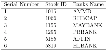
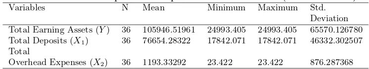
Table 1 represents the list of banks considered in this study and Table 2 presents the descriptive statistics of banks inputs and outputs used in this study below:
Table 1: List of Banks considered in this study Serial Number Stock ID Banks Name
1 1015 AMMB
Translogstochasticfron-Table 2: Banks main input and output variables 2005-2010(in RM million)
Variables N Mean Minimum Maximum Std.
Deviation Total Earning Assets (Y) 36 105946.51961 24993.405 24993.405 65570.126780 Total Deposits (X1) 36 76654.28322 17842.071 17842.071 46332.302507 Total
Overhead Expenses (X2) 36 1193.33292 23.422 23.422 876.287368
tier production model proposed by Battese and Coelli [40]. A two-step pro-cess was used to find out the technical efficiency using maximum likelihood method.The ordinary least square estimates of parameters were obtained by grid search in the first step,and then these estimates were used to estimate the maximum likelihood estimates of the parameters treated as the frontier estimates of Translogstochastic frontier production model.
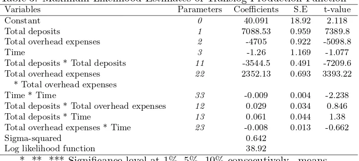
4.5 Maximum-Likelihood Estimates of Translog Production Function
The maximum likelihood estimates of the parameters of Translog stochastic frontier production model were presented in Table 3. From the analysis, we observed that the coefficients of total deposits and total overhead ex-penses were found to be significant at 1% level of significance with the values7088.530 and -4705.029respectively while the coefficient of time found insignificant with the value-1.260. The coefficient of ”total deposits” showed a positive sign, indicating that banks which use more deposits are more productive whereas the coefficient of ”total overhead expenses” showed a negative sign, indicating that banks which use less overhead expenses are more productive. We also observed that the coefficients of the squared of total deposits, total overhead expenses and time were significant at different level of significance but the interaction terms of these three input variables were insignificant.
4.6 Year Wise Mean Efficiency of Banks
Table 3: Maximum-Likelihood Estimates of Translog Production Function
Variables Parameters Coefficients S.E t-value
Constant 0 40.091 18.92 2.118
Total deposits 1 7088.53 0.959 7389.8
Total overhead expenses 2 -4705 0.922 -5098.8
Time 3 -1.26 1.169 -1.077
Total deposits * Total deposits 11 -3544.5 0.491 -7209.6
Total overhead expenses 22 2352.13 0.693 3393.22
* Total overhead expenses
Time * Time 33 -0.009 0.004 -2.238
Total deposits * Total overhead expenses 12 0.029 0.034 0.846
Total deposits * Time 13 0.061 0.044 1.38
Total overhead expenses * Time 23 -0.008 0.013 -0.662
Sigma-squared 0.642
Log likelihood function 38.92
*, **, *** Significance level at 1%, 5%, 10% consecutively, means insignificant, S.E = Standart Error
of resources.
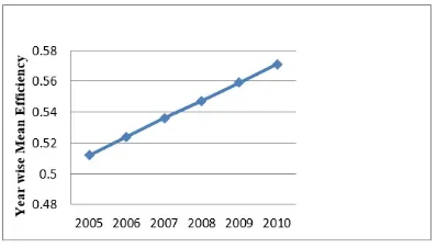
The year-wise average bank efficiency was illustrated in Table 4 and Figure 1. It was observed that on the average, bankswere 55 percent efficient on the best performing bank during the study period.In other words, the sample banks had wasted on average 45 percent of their inputs. From this investigation, we also observed that the highest average efficiency was in 2010 and the score was 57.1 percent while the lowest average efficiency was in 2005 with the score was 51.2 percent.So, the average technical efficiency score of studied six banks over the years 2005- 2010 ranges between 51 percent to 57 percent and increase over the years. Katib and Mathews [11] found that the score ranging between 68 percent and 80 percent but on a decreasing trend while Sufian [10] found Malaysian banks exhibiting 95.9 percent. From the figure 1 the overall situation of banks performance was to be clearly understood.
4.7 Year-wise Bank level Efficiency
Table 4: Year Wise Mean Efficiency of Banks Year Mean
2005 0.512 2006 0.524 2007 0.536 2008 0.547 2009 0.559 2010 0.571 Mean 0.5415
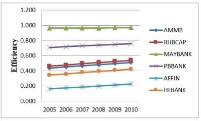
percent) AMMB (with 47.3 percent) and RHBCAP (with 50 percent). At the beginning of the study period, MAYBANK was most efficient and it retained its place at the end of the period. Similarly, AFFIN bank was least efficient and itretained its place at the end of the period. The dispar-ity between the highest efficiency (96.6 percent) and the lowest efficiency (19.4percent) was large. During the period 2005 to 2010, efficiency of all six banks was almost stable and consistent over time.Figure 2 showed a more clear perception about the performance of an individual bank.
Table 5: Year-wise Bank level Efficiency
Year AMMB RHBCAP MAYBANK PBBANK AFFIN HLBANK
2005 0.435 0.463 0.962 0.708 0.16 0.344
2006 0.45 0.478 0.963 0.719 0.173 0.36
2007 0.466 0.493 0.965 0.729 0.186 0.376
2008 0.481 0.508 0.966 0.738 0.2 0.391
2009 0.496 0.523 0.968 0.748 0.214 0.407
2010 0.51 0.537 0.969 0.757 0.228 0.423
Mean Efficiency 0.473 0.5 0.966 0.733 0.194 0.384
Figure 2: Bank level efficiency over time
4.8 Results of Hypothesis Tests
The results of various hypothesis tests were presented in Table 6. All hy-pothesis tests were obtained using the generalized likelihood-ratio statistic. The first null hypothesis is H0 :βij = 0, which showed that Cobb-Douglas
The second null hypothesis is H0 :γ = 0, which specified that there is no technical inefficiency effect in the model. As the hypothesis was rejected,we concluded that there was a technical inefficiency effect in the model.
The third null hypothesis is H0 : η = 0, which specified that the technical efficiency effect does not vary considerably over time. The null hypothesis was rejected and we can comment that the technical efficiency effect differed significantly.
Null Log-likelihood Test Critical Decision hypothesis function Statistic value*
H0:βij = 0 28.824 20.192 8.761 Reject H0
H0:γ = 0 -11.6 93.022 8.761 Reject H0
H0:η = 0 38.616 7.41 5.138 Reject H0
Notes: All
critical values are at 5% level of significance.
*The critical value is obtained from table of Kodde and Palm [41].
5. CONCLUSION
The Malaysian banking system has undergone a tremendous change during the last decade. Globalization and technological advancement has changed the way banks are operating; emphasizing the importance of mini-mizing costs and maximini-mizing profits. This study examines the efficiency of Malaysian banks listed in Kuala Lumpur Stock Exchange (KLSE) during 2005-2010 by applying a parametric frontier approach, Stochastic Frontier Approach (SFA). The average technical efficiency for Malaysian banks listed in the KLSE is 0.5415. About 55 percent of the banks have technical effi-ciency higher than the bank-industry average and about 45 percent of the banks in Malaysia listed in KLSE have less than the bank- industry average for technical efficiency. According to our results, MAYBANK and PBBANK seem to be the most efficient banks while AFFIN bank, HLBANK, AMMB and RHBCAP are the least efficient banks. Moreover, banks that made more deposits and less overhead expenses are found to be more efficient. We found that Translog Production Function is preferable than Cobb-Douglas Production Function and the level of technical efficiency has increased over the reference period.
HLBANK should act appropriately for increasing their coverage in offering innovative technology to increase their performance and raising their market competitiveness.
REFERENCES
1. Olesen, O. B., Petersen, N. C. and Lovell, C. A. K., 1996. Editors intro-duction. Journal of Productivity Analysis, 7(2/3), 87-98.
2. Berger, A. and Humphrey, D., 1997. Efficiency of financial institutions: international survey and directions for future research. European Journal of Operation Research, 98, 175-212.
3. Aigner, D., Lovell, C. and Schmidt, P., 1977. Formulation and estimation of stochastic frontier production function models. Journal of Economet-rics, 6, 21-37.
4. Meesuen, W. and Broeck, J., 1977. Efficiency estimation from Cobb-Douglas production functions with composed error. International Eco-nomic Review, 18, 435-444.
5. Berger, A.N. and Humphrey, D.B., 1991. The Dominance of Inefficiencies Over Scale and Product Mix Economies in Banking. Journal of Monetary Economics, 28(1), 117-148.
6. Berger, A.N. and Humphrey, D.B., 1992. Measurement and efficiency issues in commercial banking. InZ. Griliches, ed. Output measurement in the service sector. Chicago: University of Chicago Press, 245-279.
7. Sufian, F. and Abdul Majid, M.Z., 2007. Singapore Banking Efficiency and Its Relation to Stock Returns: A DEA Window Analysis Approach.
International Journal of Business Studies, 15(1), 83-106.
8. Li, Z., 2006. The Assessment Analysis of Efficiency of Commercial Banks Based on DEA Model, International Management Review, 2(3), 60-66.
9. Sufian, F., 2006.The Efficiency of Non-Bank Financial Institutions: Em-pirical Evidence from Malaysia. International Research Journal of Fi-nance and Economics, 6, 49-65.
10. Sufian, F., 2004. The Efficiency Effects of Bank Mergers and Acquisitions in Developing Economy: Evidence from Malaysia. International Journal of Applied Econometrics and Quantitative Studies, 1(4), 53-74.
12. Sherman, H.D. and Gold, F., 1985. Bank branch operating efficiency: Evaluation with data envelopment analysis. Journal of Banking and Fi-nance, 9, 279 - 315.
13. Aly, H.Y., Grabowski, R., Pasurka, C. andRangan, N., 1990. Technical, scale and allocative efficiencies in US banking: An empirical investigation.
Review of Economics and Statistics, 72, 211-218.
14. Elyasiani, E. and Mehdian, S.M., 1990. Efficiency in the commercial banking industry: A production frontier approach. Applied Economics, 22, 539-551.
15. Kwan, S.H. and Eisenbeis, R.A., 1996. An analysis of inefficiencies in banking: A stochastic cost frontier approach. Federal Reserve Bank of San Francisco Economic Review, No. 2.
16. Worthington , A.C., 1998. The determinants of non-bank financial insti-tution efficiency: A stochastic cost frontier approach. Applied Financial Economics.,8(3), 279-289.
17. Koetter, M., 2005. Measurement matters-input price proxies and bank efficiency in Germany, Discussion Paper Series 2: Banking and Financial Studies No. 01.
18. Lozano-Vivas, A., 1997. Profit Efficiency of Spanish Savings Banks. Eu-ropean Journal of Operational Research, 98(2), 381-394.
19. Boscia, V., 1999.The effect of deregulation on the Italian banking sys-tem: An empirical study. Research Papers in Banking and Finance, RP 98/14, School of Accounting, Banking and Economic, University of Wales, Bangor, Italy.
20. Das, A., 1997. Technical, allocative and scale efficiency of public sector banks in India. RBI Occasional Papers, 18(2&3), 279-301.
21. Kumar, S. and Satish, V., 2003. Technical efficiency, benchmarking and targets: A case study of Indian public sector banks. Prajnan, 21(4), 275-311.
22. Shanmugam, K.R. and Lakshmanasamy, T., 2001. Production frontier efficiency and measures: An analysis of the banking sector in India. Asian -African Journal of Economics and Econometrics, 1(2), 211-228.
23. Mohan T.T.R. and Ray, S., 2004. Comparing performance of public and private sector Banks: A revenue maximization approach. Economic and Political Weekly , 39(12), 1271-1275.
25. Kumbhakar ,S.C. and Subrata, S., 2003. Deregulation, ownership and productivity growth in the banking industry: Evidence from India. Jour-nal of Money, Credit, and Banking, 35(3), 403-424.
26. De, P.K., 2004. Technical efficiency, ownership and reforms: An econo-metric study of Indian banking industry. Indian Economic Review, 34(1), 261-294.
27. Sensarma, R., 2005. Cost and profit efficiency of Indian banks during 1986-2003: A stochastic frontier analysis. Economic and Political Weekly
, 40(12), 1198-1209.
28. Mahesh, H.P., and Meenakshi, R., 2006. Liberalization and productive ef-ficiency of Indian commercial banks: A stochastic frontier analysis. Manik Personal RePEc Archive Online at http://mpra.ub.uni-muenchen.de/827/ MPRA Paper No. 827.
29. Karim, M.Z.A., 2001. Comparative bank efficiency across select ASEAN countries,ASEAN Economic Bulletin, 18(3), 289- 304.
30. Fadzlan, S. and Muhd.Zulkhilbri, A. M., 2005. Post-merger banks effi-ciency and risks in emerging market: Evidence from Malaysia. The Icfai Journal of Bank Management.4(4), 16-37.
31. Hunter, W.C., Timme, S.G. and Yang, W.K., 1990. An examination of cost subadditivity and multiproduct production in large U.S. Banks.
Journal of Money, Credit, and Banking, 22, 504 - 525.
32. Battese, G.E. and Coelli, T.J., 1992. Frontier production functions, tech-nical efficiency and panel data: with application to paddy farmers in India. Journal of Productivity Analysis, 3, 153-169.
33. Kaparakis, E.I., Miller, S.M. and Noulas, A.G., 1994. Short-run cost inefficiency of commercial banks: A flexible stochastic frontier approach.
Journal of Money, Credit and Banking, 26(4), 875-893.
34. Yildirim, H.S., and Philippatos, G.C., 2002. Efficiency of banks: recent evidence from the transition economies of Europe (1993-2000), Available from URL: http://www.commerce.usask.ca/faculty/yildirim/efficiency.
35. Nikiel, E.M. and Opiela, T.P., 2002. Customer type and bank efficiency in Poland: implications for emerging market banking. Contemporary Eco-nomic Policy, 20(3), 255 - 271.
36. Lovell, C.A.K., 1993. Production frontiers and productive efficiency. In
H.O. Fried, C.A.K. Lovell, S.S. Schmidt, ed. The Measurement of Pro-ductive Efficiency. New York: Oxford University Press, 3-67.
38. Kumbhaker, S.C. and Lovell, C.A.K.,2000. Stochastic Frontier Analysis. Cambridge: Cambridge University Press.
39. Coelli, T.J., 1996. A guide to FRONTIER version 4.1: A computer program for stochastic frontier production and cost function estimation. Mimeo, Department of Econometrics, University of New England, Armi-dale.
40. Battese, G.E. and Coelli, T.J., 1988.Prediction of firm level technical efficiencies with a generalized frontier production function and panel data.
Journal of Econometrics, 38, 387-399.
41. Kodde, D. A. and Palm, A. C., 1986. Wald criteria for jointly testing equality and inequality restrictions. Econometrica, 54, 1243-1248.
MD. ZOBAER HASAN: Department of Natural Sciences, Daffodil International University, 102/1 Sukrabad, Mirpur Road, Dhanmondi, Dhaka -1207
E-mail: raihan [email protected]
ANTON ABDULBASAH KAMIL: Mathematics Section, School of Distance