www.elsevier.nlrlocaterjappgeo
Forensic GPR: finite-difference simulations of responses from
buried human remains
William S. Hammon III, George A. McMechan
), Xiaoxian Zeng
( )
Center for Lithospheric Studies, The UniÕersity of Texas at Dallas, 2601 N. Floyd Road Fa31 , P.O. Box 830688,
Richardson, TX 75083-0688, USA Received 4 April 2000; accepted 26 July 2000
Abstract
Ž .
Time domain 2.5-D finite-difference simulations of ground-penetrating radar GPR responses from models of buried human remains suggest the potential of GPR for detailed non-destructive forensic site investigation. Extraction of information beyond simple detection of cadavers in forensic investigations should be possible with current GPR technology. GPR responses are simulated for various body cross-sections with different depths of burial, soil types, soil moisture contents, survey frequencies and antenna separations. Biological tissues have high electrical conductivity so diagnostic features for the imaging of human bodies are restricted to the soilrskin interface and shallow tissue interfaces. A low amplitude reflection shadow zone occurs beneath a body because of high GPR attenuation within the body. Resolution of diagnostic features of a human target requires a survey frequency of 900 MHz or greater and an increment between recording stations of 10 cm or less. Depth migration focuses field GPR data into an image that reveals accurate information on the number, dimensions, locations and orientations of body elements. The main limitation on image quality is attenuation in the surrounding soil and within the body. 3-D imaging is also feasible.q2000 Elsevier Science B.V. All rights reserved.
Ž .
Keywords: Ground-penetrating radar GPR ; Forensic; Human remains; Finite-difference modeling
1. Introduction
Ž . Ž .
Davenport et al. 1988, 1990 and Killam 1990 discuss the applicability of ground-penetrating radar
ŽGPR and other geophysical methods to criminal.
investigations. The utility of GPR for the location of graves has been demonstrated by a number of
au-)Corresponding author.
Ž .
E-mail address: [email protected] G.A. McMechan .
Ž
thors Bevan, 1991; Unterberger, 1992; Mellett, 1992;
.
Miller, 1996; Nobes, 1999; Davis et al., 2000 . To date, successful results have been obtained indirectly by location of non-specific radar anomalies. For example, an anomaly caused by soil disturbance found during a search in a graveyard with missing headstones has a high probability of correctly indi-cating the presence of a burial. The search for a buried crime victim is more ambiguous, as the search area is necessarily larger and the presence of a burial is not positively known. The detection of an anomaly leads to a time consuming excavation to investigate
0926-9851r00r$ - see front matterq2000 Elsevier Science B.V. All rights reserved.
Ž .
( )
W.S. Hammon et al.rJournal of Applied Geophysics 45 2000 171–186
172
its nature; this is a costly and inefficient search method.
Misidentification of a GPR anomaly can cause
Ž .
problems for a criminal investigation. Mellett 1996 describes an example in which an anomaly was located beneath a concrete slab in a basement. The suspect confessed to the murder and to burying the victim in the basement. Upon excavation several years later, the detected anomaly was determined to
Ž
be a geological feature J.S. Mellett, personal
com-.
munication, 1999 . Thus, it is of importance to try to acquire and process GPR data in ways that allow extraction of more definitive information from GPR anomalies. This paper presents numerical results that imply that this is possible.
1.1. PreÕious examples
Previous work in the field of GPR grave location has concentrated in three areas: assisting in criminal investigations, forensic utility studies, and graveyard mapping. At least two murder victims have been
Ž
located using GPR Mellett, 1992; Calkin et al.,
.
1995 . GPR has also been used to map graveyards for archeological, anthropological, and historical in-vestigations. These instances are briefly described in this section to set the context for the numerical examples in the following sections.
The first instance of locating a murder victim
Ž .
using GPR, as described by Mellett 1992 , took place in March 1990. The victim had disappeared 8 years earlier, and was located with GPR at 0.5 m depth at a site that was identified by traditional techniques. The survey frequency was 500 MHz.
Ž .
Calkin et al. 1995 describe the location of a murder victim in 1992. The GPR search was con-ducted 13 months after the victim was reported missing. Available evidence suggested that the vic-tim might be buried in the basement of her house. A 500 MHz GPR survey on a grid with 0.3 m line spacing led to location of an anomaly at 0.75 m depth. Excavation produced the victim’s remains.
More recently, GPR has been used to search for suspected mass graves. Investigators used GPR to search for victims of a drug cartel in Juarez, Mexico
ŽEaton, 1999 and of a 1921 race riot in Tulsa, OK,.
Ž .
USA Nelson, 1999 .
Field tests have also been conducted in controlled
Ž . Ž
environments. Alongi 1973 analysed 1-D single
.
trace data collected over a buried dog. Strongman
Ž1992 conducted a 2-D survey over two goats and a.
bear buried at a site established to train forensic
Ž .
investigators. Roark et al. 1998 conducted a 2-D survey at a test site as part of a study of how clandestine burials change over time; two deer car-casses were the subjects of this study.
The location of graves in graveyards by GPR has
Ž .
been described in several papers. Bevan 1991 used the disturbance of soil stratigraphy to locate graves.
Ž .
Unterberger 1992 used soil disturbance and casket
Ž .
reflections to locate graves. Davis et al. 2000 de-scribe successful location of unmarked graves with a
Ž .
3-D survey in permafrost. Ivashov et al. 1998
describe the use of GPR to locate infilled excava-tions. These papers discuss detection of features that are secondary, and not unique, to the presence of a burial.
In a criminal burial, human remains are not likely to have been interred in a casket. Thus, investigators must rely on the presence of a soil disturbance or the detection of a buried object to mark the location of a burial. However, the presence of a soil disturbance does not necessarily indicate a site of interest. Nei-ther does the location of a buried object necessarily denote the presence of a human body. Thus, the ability to characterize a target using only its GPR response is potentially important to a forensic inves-tigation. For these reasons, the numerical simulation of GPR responses of human remains is a timely objective. Numerical simulations can be used to investigate the detectability of human remains under various conditions, including changing soil types and survey parameters, and also to provide test data for evaluation of data processing and imaging algo-rithms.
2. Modeling procedure
We used the 2.5-D finite-difference time domain
Ž .
Ž
superimposes 2-D responses for different
out-of-.
plane horizontal wave numbers to simulate point
Ž .
dipole sources Livelybrooks and Fullagar, 1994 ; for the examples below, we used Ks0, 2, 4, 6, and 8 my1. In the simulations, the long axes of the
transmitting and receiving dipole antennas are ori-ented parallel to each other and perpendicular to the plane of the model cross-section; this is the most common field survey configuration.
The computational grid increment in all models was ;0.29 cm in both vertical and horizontal direc-tions. Source center frequencies used were 450, 900, and 1200 MHz. The source time function was a band
Ž .
limited Ricker wavelet. A trace was saved at every sixth grid point along the airrsoil interface. The time step in all simulations was 6=10y1 2 s. These
pa-rameters correspond to a minimum of 10 grid points per wavelength at the dominant frequencies, and
Ž .w x
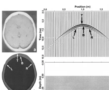
Fig. 1. Modeling for a skull cross-section. The CT image a modified from Kieffer and Hietzman, 1979 is converted into the model image Ž .b , which is then inserted into the geologic environment d . Gray levels in b and d correspond to relative dielectric permittivity valuesŽ . Ž . Ž . at 1200 MHz, as given in the legend. Transmitters and receivers are simulated at equally spaced points along the airrsoil interface. The
Ž . Ž
simulated 1200 MHz monostatic radargram c represents a shallow burial of the skull in clay-rich sand with 6.4% water content by
. Ž .
volume and is plotted with 2=the gain of the radargrams in Fig. 2. Labeled GPR waves in c are produced by the similarly labeled Ž .
( )
W.S. Hammon et al.rJournal of Applied Geophysics 45 2000 171–186
174
satisfy the stability and grid dispersion requirements
ŽPetropoulos, 1994 . The air. rearth interface was in-Ž .
serted as part of the model Fig. 1d , and Mur’s
Ž1981 second-order absorbing boundary conditions.
were used on the outer grid edges.
The models were parameterized as regions with constant values of relative dielectric permittivity and electrical conductivity for each dominant frequency
Ž .
used Table 1 . For small values of electrical
conduc-Ž . Ž .
tivity s andror high frequencies v , the relative
Ž .
dielectric permittivity ´ is the main determinant of
Ž .
the propagation velocity Õ of GPR waves:
1r2
velocity of light in vacuum e.g., Davis and Annan,
.
1989; Gueguen and Palciauskas, 1994 . The velocity
´
increases as ´ decreases, as v increases, and as s
decreases. The electrical conductivitys is the main
determinant of the attenuation of GPR waves: 35
D;
Ž .
2s
where D is the depth of penetration in meters, ands
is the conductivity at the frequency of interest in
Ž .
milliSeimensrmeter Sensors & Software, 1997 .
Values of ´ and s for all soils and tissuerbone
materials used in the models were obtained from published laboratory measurements. Gabriel et al.
Ž1996a surveyed an extensive body of literature and.
compiled dielectric properties for 13 biological tis-sues over a frequency range of 10 Hz to 10 GHz.
Ž .
Gabriel et al. 1996b conducted continuous dielec-tric measurements on 20 tissue types over the fre-quency range of 10 Hz to 20 GHz. Curtis et al.
Ž1995 made continuous dielectric measurements at.
several temperatures and moisture levels for 12 soils over the frequency range of 45 MHz to 26.5 GHz. Other sources of specific measurements used are
Ž . Ž .
Schwan and Li 1953 , Schwan and Piersol 1954 ,
Ž .
and Pethig 1979 . The values used for composite
Ž .
tissue regions Table 1 are areally weighted aver-ages of the tissues present in those model regions.
Geometries for various transverse human cross-sections were obtained from Kieffer and Hietzman
Ž1979 ; computed tomography. ŽCT. images were
Ž .
scanned from this text e.g., Fig. 1a . Each scanned CT image was then converted into an electromag-netic model by assigning the corresponding
proper-Ž .
ties Table 1 to the region containing each bone and
Ž .
tissue type and the surrounding soil Fig. 1b and d . This model was then input to finite-difference
simu-Ž .
lation to produce the GPR response Fig. 1c . The
Table 1
Ž . Ž . Ž . Ž .
The properties ´and s assigned to model regions for radargram simulation. References are: 1 Gabriel et al. 1996a , 2 Gabriel et al. Ž1996b , 3 Schwan and Piersol 1954 , 4 Schwan and Li 1953 , Pethig 1979 , and 6 Curtis et al. 1995 . Values % for the two. Ž . Ž . Ž . Ž . Ž . Ž . Ž . Ž . clay-rich sands are water content by volume
Material 450 MHz 900 MHz 1200 MHz References
Ž . Ž . Ž .
´ s Srm ´ s Srm ´ s Srm
Air 1.0 0.0 1.0 0.0 1.0 0.0 –
Clay 5.1 0.038 4.3 0.06 4.1 0.08 6
Ž .
Clay-rich sand 6.4% 3.4 0.012 3.3 0.017 3.3 0.022 6
Ž .
Clay-rich sand 25.8% 11.0 0.072 10.6 0.105 10.5 0.13 6
Dry sand 2.4 0.006 2.4 0.009 2.4 0.009 6
Skin 38.0 0.7 35.0 0.8 33.0 1.0 1,2
Bone 13.0 0.1 12.0 0.13 11.0 0.2 1–5
Ž .
Brain gray matter 60.0 0.9 50.0 1.1 45.0 1.2 1–3
White matter 47.0 0.59 45.0 0.9 40.0 1 1,2
Cartilage 48.0 0.64 45.0 0.81 40.0 0.9 2
Muscle 56.0 1.03 54.0 1.2 51.0 1.3 1–4
Bone marrow 6.0 0.075 5.5 0.1 5.0 0.115 3
Skin with fat 7.0 0.08 6.0 0.1 5.0 0.145 1–5
Liver and muscle 52.0 0.89 49.0 1.02 47.5 1.15 1–4
Table 2
The dimensions of each body section used in model generation
Model Height Width
other cross-sections were similarly constructed and modeled. The outer dimensions for each body sec-tion are listed in Table 2.
3. Modeling results
Modeling was performed for seven transverse body sections as a function of radar frequency, soil type and water saturation, burial depth, antenna sepa-ration, amount of decomposition, complexity of soil stratigraphy, and the increment between recording positions. In this section, the effect of each variable will be examined in turn.
Models are referred to by the body section and by the parameter that is varied; all other parameters are constant unless stated otherwise. All radargrams are monostatic and are plotted with the same constant gain unless stated otherwise. Plotting of all radar-grams starts at 2.5 ns as no reflections are present at earlier times for any of the models.
Fig. 2 shows synthetic radargrams for the skull
Ž .
model Fig. 1d at two frequencies and at two burial
Ž .
depths in two soil types dry sand and clay . These radargrams are used to illustrate the effects of these variables.
3.1. Effect of radar frequency
For a fixed model, the primary effects of an increase in the dominant frequency of the GPR transmitter are increases in attenuation,
resolu-Ž .
tion through an increase in bandwidth , and wave
Ž .
velocity via dispersion . Compare the 450 MHz
res-Ž .
ponses Fig. 2a and b with the 1200 MHz responses
ŽFig. 2c and d for the same model Fig. 1d . The. Ž .
frequency-dependent parameters are given in
Table 1.
Attenuation of the radar signal increases with
Ž Ž ..
increasing frequency Eq. 2 , and is greater in clay
w
than in sand because of the increased conductivity
ŽTable 1 ; compare Fig. 2a and b for sand, with Fig..x
2e and f for clay. At this plot gain, no response is visible in the 450 MHz radargram for the deep burial
Ž .
in clay Fig. 2f . Most realistic soils will produce responses between these two extremes.
The increase in GPR resolution with increasing frequency is demonstrated by comparing radargrams
Ž .
at 450 MHz Fig. 2a and b with those at 1200 MHz
ŽFig. 2c and d for the same model. The 450 MHz.
plots show only a broad reflection, but in the 1200 MHz plots, the response is resolved into at least four distinct reflections and diffractions. These arrivals are seen more clearly in the high-gain 1200 MHz response in Fig. 1c, where they are labeled and are
Ž .
seen to originate at the soilrbone T and bonerbrain
Ž .B interfaces, and at interface irregularities L andŽ .
R .
A frequency dependent increase in wave velocity
Ždispersion is indicated by two features. As fre-.
quency increases, for a given target depth and shape, the radius of curvature of the reflection hyperbola decreases and the initial arrival time of the reflected energy occurs earlier; compare Fig. 2a and c or Fig. 2b and d. Although the surrounding material
Ždry sand is the same in both models, the conductiv-. Ž .
ity changes with frequency Table 1 which changes
Ž .
the propagation velocity, via Eq. 1 .
3.2. Effect of burial depth
Fig. 2 demonstrates the effect of varying the depth of burial. In the shallow burial models
ŽFig. 2a, c, and e , the top of the target is 0.4 m.
Ž .
deep. In the deep burial models Fig. 2b, d, and f , the top of the target is 0.8 m deep. For a given target and soil type, increasing the depth of burial increases both the travel time and the attenuation because the propagation path length increases with depth. The maximum amplitude of the reflection from the
shal-Ž .
()
W.S.
Hammon
et
al.
r
Journal
of
Applied
Geophysics
45
2000
171
–
186
176
Ž .
Fig. 2. Effects of varying frequency, soil type, and burial depth. All radargrams are monostatic and are for the skull model in Fig. 1d. The upper row a, c, and e are for shallow
Ž . Ž . Ž .
burials; the lower row b, d, and f are for deep burials. The left columns a and b are 450 MHz responses for burial in dry sand. The center columns c and d are 1200 MHz
Ž .
Ž .
than that for the deep target Fig. 2b . At 1200 MHz,
Ž .
this amplitude factor is ;5 Fig. 2c and d . In clay
Ž .
at 450 MHz, this factor is ;28 Fig. 2e and f . Increasing depth of burial also increases the ra-dius of curvature of the reflections; compare Fig. 2a with b and Fig. 2c with d. For a given recording position, the reflection point moves closer to the top of a curved target as depth increases. Thus, features present in a radargram for a shallow burial will appear horizontally stretched in the radargram for a deep burial, if they are detectable at all. This
appar-ent horizontal stretching is a purely geometrical ef-fect.
3.3. Effect of soil type
Fig. 2 also demonstrates the effect of varying soil type on reflection character for the model in Fig. 1d
Žfor shallow models . Radar velocity and attenuation.
are both influenced by soil type. Dry sand has very
Ž .
low attenuation and high velocity Fig. 2a and b ;
Ž .
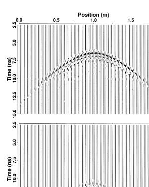
Fig. 3. The effect of varying soil water content. Both responses are for the skull model Fig. 1d in clay-rich sand at 900 MHz. Water levels
Ž . Ž . Ž . Ž . Ž .
()
W.S.
Hammon
et
al.
r
Journal
of
Applied
Geophysics
45
2000
171
–
186
178
Ž . Ž . Ž . Ž .
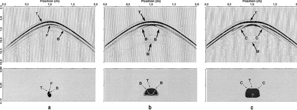
Fig. 4. Models and synthetic responses for a calf, b upper pelvis, and c lower chest sections. Gray levels in the lower model plots indicate relative dielectric permittivity Ž .
wet, clay-rich sand has very high attenuation and low
Ž .
velocity Fig. 2e and f . These represent good and poor situations, respectively, in terms of signal detec-tion. The response amplitude in clay-rich sand at 450
Ž .
MHz Fig. 2a is ;9 times smaller than that in dry
Ž .
sand at 450 MHz Fig. 2e .
3.4. Effect of soil moisture content
Fig. 3 shows the effect of varying soil water content. The model used is that in Fig. 1d; the surrounding soil is clay-rich sand. Responses for 6.4% and 25.8% volumetric water content in the soil are shown in Fig. 3a and b, respectively. The in-crease in soil water content results in an inin-crease in
attenuation and a decrease in signal velocity. The maximum amplitude of the response of the drier
Ž6.4% water model is. ;33= that of the wetter Ž25.8% water model. The low. ´ values measured
for these samples are a consequence of the high clay fraction; water absorbed by clay has significantly
Ž
lower ´ than free water Curtis et al., 1995; Wang
.
and Schmugge, 1980 .
3.5. A selection of profiles; simulations and migra-tions
Fig. 4 contains models and simulated monostatic GPR profiles for calf, upper pelvis, and lower chest
Ž . Ž . Ž .
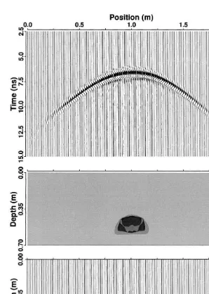
Fig. 5. Composite model b is for a section through the upper chest and arms. a is the simulated monostatic 900 MHz GPR response; c
Ž . Ž . Ž .
is a after depth migration. a is plotted using the same gain as Fig. 2; c is plotted with 70=lower gain. High amplitudes are clipped. Ž .
( )
W.S. Hammon et al.rJournal of Applied Geophysics 45 2000 171–186
180
body sections. All three simulations are for shallow burials in dry sand at 900 MHz. Responses were also
Ž .
computed but not shown here for a series of partial models in which layers were added one at a time. This procedure allowed identification of the origin of each of the individual reflections in the full model responses, as labeled in Fig. 4.
Figs. 5, 6, and 7 contain simulated radargrams for three models and their corresponding migrated sec-tions. All models represent shallow burials in
clay-Ž .
rich sand with 6.4% water and all simulations are for 900 MHz. Migration was performed using a
Ž
seismic frequency–wave number algorithm Stolt,
.
1978 which was modified for use with GPR data
Ž . Ž . Ž . Ž .
Fig. 6. Model b is for a section through the lower pelvis. a is the simulated monostatic 900 MHz GPR response; c is a after depth
Ž . Ž .
migration. a is plotted using the same gain as Fig. 2; c is plotted with 70=lower gain. High amplitudes are clipped. Refer to Fig. 1b for Ž .
Ž . Ž . Ž . Ž .
Fig. 7. Composite model b is for a section through the thighs. a is the simulated monostatic 900 MHz GPR response; c is a after depth
Ž . Ž .
migration. a is plotted using the same gain as Fig. 2; c is plotted with 70=lower gain. High amplitudes are clipped. Refer to Fig. 1b for Ž .
the permittivity scale used to plot b .
ŽSensors & Software, 1996 . Migration moves the.
recorded reflected and diffracted waves from the receiver locations back to where they were originally scattered in space, to form a focussed image of the target. The migrated images contain more accurate information on the number, locations, dimensions and orientations of the body elements than the recorded unmigrated data do.
Fig. 8 shows a psuedo 3-D composite body image produced by placing 10 migrated 2-D body sections in their correct relative positions for perspective. The body outline and contours are visible; higher resolu-tion could be achieved with higher frequencyr band-width data, but Fig. 8 is a realistically obtainable representation.
3.6. Effect of antenna separation
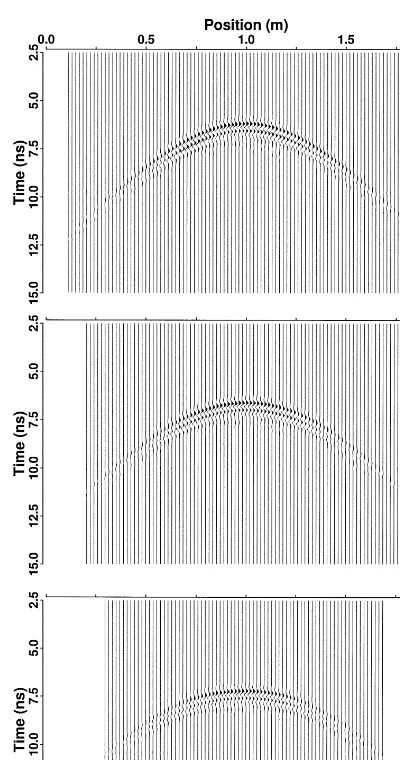
Fig. 9 shows the effect of varying the transmitter-to-receiver antenna separation during data acquisi-tion. The model used is that in Fig. 1d. The effect of increasing antenna separation is similar to increasing burial depth; arrival times increase as antenna sepa-ration increases because of the increase in path lengths. Apparent horizontal stretching occurs simi-lar to that described above for increasing target depth.
( )
W.S. Hammon et al.rJournal of Applied Geophysics 45 2000 171–186
182
Fig. 8. A pseudo 3-D composite of migrated body cross-sections. The rectangle is a transparent plane parallel to the radargram sections,
Ž .
containing the fourth cross-section from the bottom that labeled pelvis , as reference for the 3-D view perspective. Labels indicate the body sections imaged by the corresponding radargram.
Ž
angle of maximum antenna radiation which is equal
.
to the critical refraction angle at the earth’s surface . Amplitudes increase and then decrease locally as the maximum radiation angle is encountered as a survey line passes over a target. This pattern may make certain features more or less visible, depending on the angle and the target depth.
3.7. Effects of adÕanced decomposition
Fig. 10a shows the effect that decomposition has on the character of the skull radargram. The decom-posed model was constructed by substituting soil for the skin layer and air for the brain tissue. This is assumed to simulate the decomposed state of the human skull. All other parameters, except the plot-ting gain, are the same as in Fig. 1c.
The radargram for the decomposed specimen con-tains reflections from the base of the skull, as well as internal reflection multiples. None of the fresh speci-men radargrams contain visible basal reflections due to the very high GPR attenuation in body tissues. The maximum reflection amplitude from the decom-posed specimen model is 60% greater than that from
the equivalent fresh specimen model. The substitu-tion of air for brain tissue results in greater dielectric permittivity and electrical conductivity ratios at the bone to skull cavity interface. The resulting higher net reflectivity causes the difference in amplitude.
3.8. Effects on responses from underlying soil stratigraphy
Fig. 10b demonstrates the effect that a buried body would have on the 900 MHz response of underlying soil stratigraphy. This model is the same lower chest section as in Fig. 4c, with the addition of
Ž .
a wet 25.8% water by volume , clay-rich sand layer at a depth of 0.7 m.
Ž .
The main slightly flattened hyperbolic reflection
Ž .R in Fig. 10b is the response from the chest. The
Ž .
planar reflection S is from the interface between
Ž . Ž .
the two soil types; the gap G in S is a low
amplitude shadow caused by signal attenuation in the chest. Once the signal has passed through the body, it is attenuated beyond the threshold of detection.
Ž .
discontinu-Fig. 9. Effects of varying antenna separation. The separations are Ž .a 20 cm, b 40 cm, and c 60 cm. See Fig. 1c for 0 cmŽ . Ž . separation. The horizontal axis gives the position of the midpoint between the two antennas. Profiles are plotted with the same gain as Fig. 2.
ous reflector. The latter explanation is clear because the diffractions are one-sided, being attenuated be-neath the body; a discontinuous reflector would pro-duce two-sided diffractions emanating from the points of truncation.
3.9. Effects of surÕey stepsize
Fig. 10c shows the effect of varying survey step-size. In this 900 MHz radargram, the trace spacing is 9.25 cm; for comparison, these are the same data as
in Fig. 3a, but with only every fifth trace plotted. The same general features can be recognized in both radargrams. However, the data in Fig. 10c are spa-tially aliased beyond the center five traces, which limits the types of processing that can be done.
Ž . Fig. 10. The effects on data for the skull model of Fig. 1d of a
Ž .
advanced decomposition, b the presence of soil stratigraphy, and Ž .c a 9.25 cm stepsize between traces. a and c are plotted withŽ . Ž .
Ž .
the same gain as Fig. 2. b is plotted at 0.5=the gain of Fig. 2. Ž .
High amplitudes are clipped. In a , T is the reflection from the skull top, B is the reflection from the skull bottom, and M is the
( )
W.S. Hammon et al.rJournal of Applied Geophysics 45 2000 171–186
184
Table 3
Ž .
Estimated GPR resolution at normal incidence in body tissues; values listed are calculated one-quarter wavelengths
Body tissue 450 MHz 900 MHz 1200 MHz Žcm. Žcm. Žcm.
Liver, lung, 2.4 1.3 0.9
and muscle
3.10. Resolution
Ž .
Table 3 lists the resolution at normal incidence of various radar frequencies in the major body
tis-Ž
sues. The very high permittivity values and hence,
.
low velocities of biological tissues result in higher resolution than in the surrounding soils for a given frequency; very small-scale features within the hu-man body can produce diagnostic reflections. How-ever, the high conductivity of tissues makes the detection of any features more than a few centime-ters beneath the upper surface of the body unlikely
ŽEq. 2 .Ž ..
4. Discussion and conclusions
GPR has been used to locate buried human re-mains under a variety of circumstances. To date, this work has relied primarily on the location of non-specific and non-diagnostic GPR anomalies. This paper demonstrates the potential ability of GPR to resolve diagnostic features of the human body. It also shows the limitations of GPR for this applica-tion.
GPR frequencies must be 900 MHz or greater to resolve details within the human body. At these frequencies, resolution is better in biological tissue than in soils. However, signal attenuation also be-comes a serious problem at these frequencies. GPR performs best in drier, sandier soils. Lower frequen-cies may be required to detect burials in wetter, or more clay-rich soils. High resolution may only be
possible at shallow depths. Fortunately, criminal
Ž .
burials are typically shallow ;0.5 m . The prob-lems listed above can be partially alleviated by in-creasing the number of traces that are stacked at each survey point during acquisition, to improve the sig-nal-to-noise ratio.
Only the upper layers of the human body produce detectable GPR reflections because of the extremely high electrical conductivity of biological tissues. The resulting high attenuation produces a signal shadow and associated diffraction tails beneath the body. The GPR profiles for most body cross-sections are ex-pected to contain responses mainly from the upper soilrtissue interface. Deeper burials will produce responses that are horizontally stretched with respect to shallow responses.
The radargrams presented above should be con-sidered only as a general guide for interpretation and as a demonstration of application potential. The hu-man body varies significantly in morphology along its longitudinal axis; our 2-D modeling ignored these variations. For instance, a radargram imaging a hu-man skull would normally also contain off-line re-flections from the shoulders; thus, real data would be more complicated than the synthetic data presented here. However, the main conclusions will also hold true for real data.
During modeling, the organs of the chest and abdominal cavity were treated as a single homoge-nous mass. The permittivity and conductivity as-signed to each abdominal or chest section was an areally weighted average of the values of the organs present in that profile. This was done to keep the complexity of the models within reasonable limits. These organs, for the most part, have similar dielec-tric behavior. However, reflections from the ab-domen of a real body would be more complex than those shown here.
The modeled radargrams will also only be consis-tent with real data for some time after death and burial. A significant change in radargram character will take place with the collapse of the abdominal cavity. Depending on depth of burial and other pa-rameters, this occurs ;6–12 months after death
ŽRodriguez and Bass, 1985; Galloway, 1997;
Ro-.
the abdomen and proximal sections. Eventually, the body will become completely skeletonized. When this occurs, the ribs collapse and the pelvis flattens. By this time, very little of the data presented above would be pertinent. However, the numerical simula-tion technique used here is equally applicable to all such situations. Such modeling would also be useful for archeological, anthropological, and historical ap-plications and is a topic for future research.
Data acquisition in the past was characterized by the use of relatively low frequencies in continuous
Ž
survey profiles. A stepped survey recording at a
.
series of discrete points provides more accurate and diagnostic data than a continuous survey because of less lateral smearing and the ability to stack traces at each survey point to increase the signal-to-noise ratio. Determination of diagnostic features for an imaged human target requires a survey frequency of 900 MHz or greater and a survey stepsize of 10 cm or less. Such a small stepsize would result in a time consuming survey and thus, is not well suited to a broad reconnaissance survey, but is ideal for detailed investigation of candidate sites identified by other more traditional means.
Acknowledgements
The research leading to this paper was supported by the sponsors of the UT-Dallas GPR Consortium. The authors would like to thank Lippincott, Williams, and Wilkins for permission to reproduce the skull CT scan in Fig. 1a. This paper is contribution No. 925 from the Geosciences Department at the Univer-sity of Texas at Dallas.
References
Alongi, A.V., 1973. A short-pulse high-resolution radar for ca-daver detection. Proceedings, 1st Intl. Electr. Crime Counter-measures Conf.. pp. 79–87.
Bevan, B.W., 1991. The search for graves. Geophysics 56, 1310– 1319.
Calkin, S.F., Allen, R.P., Harriman, M.P., 1995. Buried in the basement: geophysics role in a forensic investigation. Proceed-ings, SAGEEP, Environ. Eng. Geophys. Soc.. pp. 397–403. Curtis, J.O., Weiss, C.A., Everett, J.B., 1995. Effect of soil
composition on complex dielectric properties. US Army Corps Eng. Waterways Exp. Station, Tech. Rep. EL-95-34. Davenport, G.C., Griffin, T.J., Lindemann, J.W., Heimmer, D.,
1990. Geoscientists and law enforcement professionals work Ž .
together in Colorado. Geotimes 35 7 , 13–15.
Davenport, G.C., Lindemann, J.W., Griffin, T.J., Borowski, J.E., 1988. Crime scene investigation techniques. Leading Edge 7 Ž .8 , 64–66.
Davis, J.L., Annan, A.P., 1989. Ground penetrating radar for high resolution mapping of soil and rock stratigraphy. Geophys. Prospect. 37, 531–551.
Davis, J.L., Heginbottom, J.A., Annan, A.P., Daniels, R.S., Berdal, B.P., Bergan, T., Duncan, K.E., Lewin, P.K., Oxford, J.S., Roberts, N., Skehel, J.J., Smith, C.R., 2000. Spanish flu victims in permafrost. J. Forensic Sci. 45, 68–76.
Eaton, T., 1999. Grave site at Juarez searched. Dallas Morning Ž .
News 151 62 , 1A.
Gabriel, C., Gabriel, S., Corthout, E., 1996a. The dielectric prop-erties of biological tissues: I. Literature survey. Phys. Med. Biol. 41, 2231–2249.
Gabriel, S., Lau, R.W., Gabriel, C., 1996b. The dielectric proper-ties of biological tissues: II. Measurements in the frequency range of 10 Hz to 20 GHz. Phys. Med. Biol. 41, 2251–2269. Galloway, A., 1997. The process of decomposition: a model from the Arizona–Sonoran Desert. In: Haglung, W.D., Sorg, M.H. ŽEds. , Forensic Taphonomy, The Postmortem Fate of Human. Remains. CRC Press, pp. 139–150.
Gueguen, Y., Palciauskas, V., 1994. Introduction to the Physics of´ Rocks. Princeton Univ. Press.
Ivashov, S.I., Sablin, V.N., Sheyko, A.P., Vasiliev, I.A., Isaenko, V.N., Konstantinov, V.F., 1998. GPR for detection and mea-surement of filled up excavations for forensic applications. Proceedings, 7th International Conference on Ground Penetrat-ing Radar, University of Kansas. pp. 87–89.
Killam, E.W., 1990. The Detection of Human Remains. Charles C. Thomas, Springfield, IL.
Kieffer, S.A., Hietzman, E.R., 1979. An Atlas of Cross-Sectional Anatomy. Harper & Row, Hagerstown, MD.
Livelybrooks, D., Fullagar, P.F., 1994. FDTD2Dq: a finite-dif-ference, time-domain radar modeling program for two-dimen-sional structure. Proceedings, 5th International Conference on Ground Penetrating Radar, University of Waterloo. pp. 87– 100.
Mellett, J.S., 1992. Location of human remains with ground-penetrating radar. Proceedings, 4th International Conference on Ground Penetrating Radar, Geol. Surv. Finland. pp. 359– 365.
Mellett, J.S., 1996. GPR in forensic and archeological work: hits and misses. Proceedings, SAGEEP, Environ. Eng. Geophys. Soc.. pp. 487–491.
Miller, P.S., 1996. Disturbances in the soil: finding buried bodies and other evidence using ground penetrating radar. J. Forensic Sci. 41, 648–652.
Mur, G., 1981. Absorbing boundary condition for the finite-dif-ference approximation of the time-domain electromagnetic field equations. IEEE Trans. Electr. Comp. EMC-23, 377–382. Nelson, M., 1999. Burial site may be link to 1921 riot. Daily
( )
W.S. Hammon et al.rJournal of Applied Geophysics 45 2000 171–186
186
Nobes, D.C., 1999. Geophysical surveys of burial sites: a case study of the Oaro urupa. Geophysics 62, 357–367.
Pethig, R., 1979. Dielectric and Electronic Properties of Biologi-cal Materials. Wiley, New York.
Petropoulos, P.G., 1994. Stability and phase error analysis of FD-TD in dispersive dielectrics. IEEE Trans. Antennas Propag. 42, 62–69.
Roark, M.S., Strohmeyer, J., Anderson, N., Shoemaker, M., Op-pert, S., 1998. Application of the ground-penetrating radar technique in the detection and delineation of homicide victims and crime scene paraphernalia. Proceedings, SAGEEP, Envi-ron. Eng. Geophys. Soc.. pp. 1063–1071.
Rodriguez, W.C., 1987. Decomposition of buried and submerged Ž .
bodies. In: Haglung, W.D., Sorg, M.H. Eds. , Forensic Taphonomy, The Postmortem Fate of Human Remains. CRC Press, pp. 459–467.
Rodriguez, W.C., Bass, W.M., 1985. Decomposition of buried bodies and methods that may aid in their location. J. Forensic Sci. 30, 836–852.
Sensors & Software, 1996. PulseEKKO 2-D F-K migration. Tech-nical Manual vol. 26.
Sensors & Software, 1997. EKKO Update. January.
Schwan, H.P., Li, K., 1953. Capacity and conductivity of body tissues at ultrahigh frequencies. Proc. I.R.E. 41, 1735–1740. Schwan, H.P., Piersol, G.M., 1954. The absorption of
electromag-netic energy in body tissues. Am. J. Phys. Med. 33, 371–404. Stolt, R.H., 1978. Migration by Fourier transform. Geophysics 43,
23–48.
Strongman, K.B., 1992. Forensic applications of ground penetrat-ing radar. Proceedpenetrat-ings, 2nd International Conference on Ground Penetrating Radar, Geol. Surv. Canada. pp. 203–211, Paper 90-4.
Unterberger, R.R., 1992. Ground penetrating radar finds disturbed earth over burials. Proceedings, 4th International Conference on Ground Penetrating Radar, Geol. Surv. Finland. pp. 351– 357.
Wang, J.R., Schmugge, T.J., 1980. An empirical model for the complex dielectric permittivity of soils as a function of water content. IEEE Trans. Geo. Remote Sens. GE-18, 288–295. Xu, T., McMechan, G.A., 1997. GPR attenuation and its