Constraints For Government Monetary
And Debt Policy*
William B. English
Some economists have pointed to credit constraints as possible explanations for two phenomena. First, credit constraints could explain violations of Ricardian equivalence. Second, constraints could also provide a mechanism through which monetary policy could affect the real economy independent of effects on interest rates. Hayashi (1986) shows that some types of credit constraints do not necessarily imply a violation of Ricardian equivalence. Similarly, this paper finds that the effects of government monetary and debt policies in an economy characterized by credit constraints can be similar to those in a model without constraints. © 2000 Elsevier Science Inc.
Key Words:Credit rationing; Monetary policy; Debt policy
JEL Classification:E44
I. Introduction
Macroeconomists have appealed to credit “constraints” or credit “rationing” in order to explain two observations. The first observation is that agents do not appear to smooth consumption optimally over time, as they should according to the Life Cycle-Permanent Income model of consumption [Hall and Mishkin (1982)]. One consequence of their failure to do so is that debt-financed tax cuts may have effects on agents’ levels of consumption and savings—i.e., Ricardian equivalence may fail [Poterba and Summers
Board of Governors of the Federal Reserve System, Division of Monetary Affairs, Washington, D.C., USA Address correspondence to: Dr. W. B. English, Board of Governors of the Federal Reserve System, 20th and C Streets, NW, Washington, D.C. 20551.
*The analysis and conclusions in this paper are mine alone and do not indicate concurrence by other members of the research staffs, by the Board of Governors, or by the Federal Reserve Banks. I thank the anonymous referee and seminar participants at the University of Pennsylvania and the Federal Reserve Board for useful suggestions. Stan Fischer, Fumio Hayashi, and Olivier Blanchard provided useful comments on much earlier drafts of this paper. All remaining errors are mine.
(1987)]. The second observation is that changes in the user cost of capital appear to have very small effects on aggregate investment spending while simple accelerator models perform fairly well [Clark (1979); Clark (1993)]. In addition, a number of papers in recent years have found that measures of internal funds seem to have a substantial impact on investment spending for at least some firms (e.g., Fazzari et al. (1988); Hubbard et al. (1995)]. These results suggest that some firms are credit constrained, and some econo-mists have argued that monetary policy could have direct effects on output by relaxing rationing constraints [Blinder and Stiglitz (1983); Stiglitz (1987); see also Jaffee and Stiglitz (1990)].1Hayashi (1985) casts doubt on the first of these uses of credit rationing. He shows that agents who are constrained in the sense that they appear to violate the usual Euler equation tests of the Life Cycle-Permanent Income Hypothesis may not increase their consumption spending in response to a debt-financed tax cut. Hayashi concludes that the implication of credit constraints for Ricardian equivalence depends heavily on the way that they are modeled. [Yotsuzuka (1986) finds a similar result.]
This paper questions the second of these uses of credit rationing. I construct a simple general equilibrium model in which agents are constrained in the credit market. Then I consider the effects of changes in monetary policy on the steady states of the model. I find that the credit constraints do not imply that changes in monetary policy have direct quantity effects. Instead, changes in government policy have effects similar to those in models without rationing. I conclude that the effects of credit constraints on the impact of monetary policy depend on what sorts of credit constraints are present.
In this paper, I employ a model of what Keeton (1979) calls “type 1” rationing very similar to those employed in de Miza and Webb (1992) and Gray and Wu (1995). In this model individual loans become riskier as they get larger. As a result, if the loan market is competitive and the quantity borrowed is observable, borrowers find that they have to pay a higher interest rate in order to increase the size of their loan. In the resulting equilibrium borrowers would choose to borrow more at the agreed upon interest rate. It is in this sense that credit is rationed.
In order to consider the effects of government policy, I embed the credit rationing model in a general equilibrium overlapping generations model. Unlike Smith (1983), who uses an endowment model, my model includes physical investment, allowing me to analyze the effects of government policy and rationing on investment and output. Fol-lowing Romer (1985), I use a simple storage technology, rather than a production function including capital and labor, to model investment opportunities. Unlike Romer’s model, the returns on investment in this model are uncertain. In order to generate a demand for money, I impose a simple financial structure, similar to that of Romer’s “pure banking economy.” There is a banking sector that intermediates between borrowers and lenders. The government supplies fiat money to satisfy a reserve requirement, and it can also issue government debt. The overlapping generations structure is convenient for two reasons. First, because agents only live for two periods, I do not need to consider reputation effects in the credit market. Second, because the model is a completely specified general equilibrium model, I can consider the welfare effects of different government policies.
1This view goes back at least to the “availability doctrine” of Roosa (1951), a modern presentation of which
The analysis proceeds in two directions. First, I consider positive issues. I characterize the steady-state, and derive the effects on steady-state interest rates and investment of changes in the government policy variables. The policy variables that I consider are the required reserve ratio, the rate of growth of high-powered money, and the level of government debt. As in Romer (1985), these comparative steady state results correspond to the effects of an unanticipated, permanent, change in the parameters (leaving aside the effects on the initial old).
The second set of issues I consider are normative. I derive the policies that the government should pursue to maximize social welfare. These optimal policies reflect the Diamond (1965) dynamic efficiency result. I then consider the welfare implications of the rationing. I find that rationing raises welfare relative to an alternative equilibrium in which rationing does not occur.
Finally, I note that deposits would be dominated if costless private lending were possible. By introducing a costly technology for private loans, I am able to construct a model in which bank lending and a private bond market coexist. Using this more complex model, I find that many of the results obtained with the simple model continue to hold. The first section of the paper presents the model and displays its steady-state condi-tions. The second section presents the effects on the steady state of the model of changes in government policy variables, and the third section addresses the welfare effects of policy. A model with a more complex financial structure is discussed in the fourth section. A final section provides some concluding remarks.
II. The Model
The economy consists of overlapping generations of two-period lived individuals. Each individual has an endowment,w, when young. The distribution of the endowments across the members of each generation is given byf(w), wherewranges from 0 toW, and over that rangef(w)is continuous and strictly positive. Individuals are risk-neutral, and choose to consume only when old. They have two ways to transfer wealth from one period to the next. First, they can invest in a risky storage technology, perhaps augmenting their endowment by borrowing in order to increase the size of the investment. Second, they can make a deposit at a bank and receive a risk-free real return,rD. (No loans directly from one person to another are allowed until Section IV).
The Storage Technology
Returns on storage display stochastic decreasing returns to scale. An investment of sizeI in the storage technology succeeds with a probabilityP(I), and fails with a probability 1-P(I). The probability of success declines with project size. The project yields (11rˆ)Iif successful, and zero if unsuccessful.2Thus, the expected return on a project of size
Iis:
R~I!;P~I!~11rˆ!I
2 This setup is somewhat simpler than those in de Miza and Webb (1992) and Gray and Wu (1995). Both
I assume that the expected return is a twice continuously differentiable function of project size, with:
R9~I!.0 and
R0~I!,0
Banks
Banks are risk-neutral, competitive intermediaries (or are so large that the risk from an individual loan is completely diversified). Banks’ intermediation services are assumed to be costless. They accept deposits from individuals and invest these funds in two assets: currency, which they hold to satisfy a reserve requirement; and loans to individuals. The required reserve ratio isf. The only role for currency in the model is as reserves for the banks. I assume that the return on loans dominates that on currency in equilibrium, and so banks do not choose to hold excess reserves. Indeed, the requirement that banks hold reserves serves as a tax on intermediation, and so risk-neutral individuals will not choose to both borrow and hold deposits. Thus, an individual with an endowment w that chooses to borrowL from a bank will investw 1 L in the storage technology. In the event of failure, the bank gets nothing. Thus, for a given real interest rate on a loan,rL; endowment size,w; and loan size,L; the bank’s expected return on a loan is:3
P~w1L!~11rL!
In order to make a loan, banks must raise 1/(12f) of deposits and hold reserves of f/(12 f) for each unit of loan. Thus, the cost of funding a loan is:4
1
12f ~11r
D!2 f
12f
S
1 11pDwherepis the inflation rate during the term of the loan, which is assumed known when the loan is made, and the second term takes account of the real cost of holding reserves. It is convenient to definerto be the real cost of loanable funds to the bank:
11r;1 1
2f ~11r
D!2 f
12f
S
111pD (1)
Because banking is competitive, the bank must earn an expected rate of return on loans that is equal to the cost of funding them:
11r 5P~w1L!~11rL!
Solving this equation, one gets the rate banks will charge on a loan as a function ofr,w, andL:
11rL5 11r
P~w1L! (2)
3I assume thatrˆis greater thanrL, so that the loan is paid in full so long as storage is successful.
Note that, for a given endowment size, the loan interest rate is an increasing function of the size of the loan,L.
The Individuals’ Problem
Because individuals are risk-neutral and only consume in the second period of life, their optimization problem amounts to maximizing expected second period consumption by choosing levels of deposits, borrowing, and storage. Because of the stochastic decreasing returns to storage, individuals with small endowments will want to borrow from banks while those with large endowments will want to deposit funds with banks. As noted earlier, it will never be optimal for an individual to both hold deposits and borrow, because doing so means that the individual’s expected consumption is reduced by the amount of the reserve tax.
The optimization problem for a borrower is given by:
Maximize: L,rL
R~w1L!2P~w1L!~11rL!L
subject to equation (2). Because projects get riskier as they get larger, the loan supply curve facing the borrower slopes upward.5The first-order conditions are the constraint,
and, after substituting for the Lagrange multiplier:
R9~w1L!5~11r!
In words, the marginal expected return on investment must equal the bank’s opportunity cost of funds. The second-order condition for a maximum is:
R0~w1L!,0
which is satisfied given our assumptions aboutR(I).
There are two characteristics of this result worth noting. First, the borrower does not choose the size of the loan given the loan interest rate, instead, both the size of the loan and the loan rate are chosen subject to the bank’s zero-profit condition. Thus, both the size of the loan and the loan interest rate are functions of the bank’s cost of funds,r. As a result, the borrower does not receive the quantity of funds that would be demanded at the contracted loan rate. The borrower’s demand curve is the solution of:6
Maximize: L
R~w1L!2P~w1L!~11rL!L
The first-order condition for this unconstrained problem is:
R9~w1L!2P~w1L!~11rL!2P9~w1L!~11rL!L50 The second-order condition for a maximum is:
5The borrower’s problem looks similar to that of a monopsonist. It is not the same, however, because there
are many borrowers, each assumed small with respect to the bank. As Keeton (1979, Chapter 1) points out, credit is a non-homogeneous good in this case.
6Note that the borrower will never choose to borrow and deposit funds rather than invest them in the storage
technology. Doing so would yield a payoff of rD per dollar in non-default states, but costrLper dollar in
non-default states. In default states the borrower gets nothing in any case. BecauserDis less thanrL, this strategy
R0~w1L! rˆ2r
L
11rˆ 1P0~w1L!~11r
L!w,0
which is assumed to hold. (Because R0 is negative, a sufficient (but not necessary) condition for the second-order condition to hold is thatP0be negative.) If the second-order condition does not hold, then it is optimal to borrow an unbounded amount from banks in order to invest.
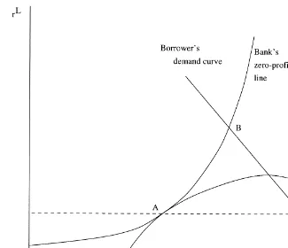
The first-order condition implies that the demand curve intersects the borrower’s isoutility lines at the point at which their slope is zero. Figure 1 shows the optimal (L,rL) as well as the borrower’s loan demand curve takingrLas given. The optimum is at the point where the borrower’s isoutility line is tangent to the bank’s zero-profit line. It is clear that a contract at pointB, the intersection of the supply and demand curves, is strictly worse for the borrower than the optimal solution at pointA. It is also clear that, given the interest rate at pointA, the borrower’s demand for credit is at pointC. It is in this sense that there is rationing in the credit market.
The second characteristic is that the optimal project size is independent of the size of the agent’s endowment. The first-order condition can be rewritten as:
R9~I*!511r (3)
whereI* is the optimal project size. Thus, the borrower’s optimal loan size can be written as:
L*~r,w!5I*~r!2w
Because all borrowers have the same project size, the interest rate on all loans will be the same and will be given by:
11rL5 11r
P~I*~r!! (4)
In contrast to those with small endowments, who borrow to invest, those individuals with large endowments may choose to invest a portion of their endowments in financial assets, in this model either bank deposits or government debt. Because deposits and government debt are both riskless assets, and there are no nonpecuniary benefits to holding deposits (no transactions services for example), the two assets must have the same return (i.e.,rD5rB). The choice of optimal storage size is a simple one:
Maximize: I
R~I!1~11rD!~w2I!
The first-order condition for this problem is:
R9~I**!511rD (5)
whereI**(rD) is the optimal amount of storage, given rD, and the optimal amount of financial assets isw2I**(rD). The first-order condition makes sense, as it means that the marginal expected return on storage is set equal to the return available on financial assets. To summarize, individuals with endowments of less than I*(r) borrow funds from banks in order to investI* in the storage technology. By doing so, they equalize their marginal return on storage and the marginal cost of funds, where the marginal cost is not the loan interest rate, but rather the cost of funds that banks face when making loans,r. Individuals with endowments betweenI*(r) andI**(rD) simply invest their endowment in the storage technology. Individuals with endowments larger than I** invest I** in the storage technology and deposit the rest. Doing so equalizes their marginal return on storage and the deposit interest rate.
Given the distribution of endowments across the young cohort, f(w), the average demand for loans per member of the young cohort as a function of banks’ cost of funds can be written as:
L~r!5
E
0
I*~r!
~I*~r!2w!f~w!dw (6)
At the same time, the supply of deposits to the banking sector per member of the young cohort as a function of the deposit rate can be written as:
D~rD!5
E
I**~rD!W
~w2I**~rD!!f~w!dw (7)
The Government
The government has three roles in the model. First, it supplies high-powered money—i.e., reserves—to the banks. The real amount of high powered money per member of the young cohort isHt.
7The government is assumed to increase the nominal supply of high-powered
money each period at a constant rate h. Second, the government supplies bonds, paying an interest ratert
B, to individuals. The real stock of bonds per member of the young cohort is assumed fixed at B. Third, government takes the resources that it receives from these activities and spends them on real per capita government spending,Gt. The individuals’ utility is not affected by the level of government spending. By assumption, the govern-ment does not produce anything itself, and so must generate a non-negative level of revenues.
The government receives a real flow of resources each period of:
h 11pt
Ht21
~11n!1B
where n is the constant growth rate of the young cohort. The first term is the real value (per member of the young cohort) of the increase in the nominal money supply. The second term is the new issuance of government debt. The government’s use of resources each period is:
Gt1~11rt21
B ! B
11n
where the first term is government spending and the second is the payments of principal and interest on the previous period’s stock of bonds. And so the government’s budget constraint each period is:
Gt1
rtB21B
11n5 h 11pt
Ht21
~11n!1
n
11nB (8)
where the left hand side is government spending on goods and on debt service, while the right-hand side is revenue from seigniorage and from new borrowing.
7 Because the government budget accounting depends on changes in money and debt over time, it is
Equilibrium
A perfect foresight competitive equilibrium for this economy consists of sequences for prices (rD,rB,rL, and the price level,P) and real quantities [D(w),L(w),I(w),H, andG], such that [D(w), L(w), and I(w)] solve the maximization problem of young households having endowment w given the prices; [D(w),L(w), andI(w)] satisfy the banks’ zero profit condition for a loan to an individual with endowment w given the prices; (G,H, andB) satisfy the government’s budget constraint given the prices; and the markets for credit, money, and goods all clear.8
Steady-State Conditions
Let the steady-state values ofrD,rB,rL,p,D(w),L(w),I(w),H,G, be indicated by bars, r
#D, etc. Leaving aside asymptotically non-monetary equilibria, the economy jumps im-mediately to this steady state. This immediate adjustment is possible because there is no long-lived capital in the model. Each generation can choose its own level of storage independent of the level chosen by its predecessor. One implication of this technology is that the comparative steady state effect of a change in government policy is the same as the effect of an unexpected change in policy except for the effect on the old generation at the time of the policy change.
Credit market. Borrowing by low-endowment individuals and the government must equal high-endowment individuals’ holdings of financial assets (deposits and bonds), less the portion banks hold as required reserves:
L~r#!1B5D~r#D!2f~D~r#D!2B!
Thus, credit market equilibrium in steady state implies that
D~r#D!5 1
12f L~r#!1B (9)
The left-hand side of equation (9) is the supply of savings. The right-hand side is the demand for savings by individuals and the government. The 1/(12f) term is necessary to take account of the fact that banks need to raise 1/(12f) of deposits in order to fund a unit of loans because of the reserve requirement.
The banks’ zero profit condition links r#, and r#D:
11r#5 1
12f ~11r#
D!2 f
12f
S
111p#
D
(10)The equilibrium in the credit market can be displayed graphically by substituting equation (10) in the right-hand side of equation (9), and plotting the supply and demand for funds as functions ofr#D, as shown in Figure 2. The intersection of supply and demand yields the steady-state value of the deposit rate.
8As one might expect, there could be many equilibria of this model in which value of the real per capita
Money market. The only demand for money in the economy is the demand for reserves:
H# 5f~D~r#D!2B! (11)
In the steady state, the real stock of money per member of the young cohort is constant. With constant growth of the nominal money supply at rate hand constant population growth at raten, the steady-state inflation rate is given by:
11p# 511h
11n (12)
Goods market. If the money and credit markets clear, then Walras’ law implies that the goods market must also clear. In the steady state, government spending is constant and is given by:
G# 5 h 11p#
H#
11n1~n2r#
B! B
11n (13)
This value ofG# is assumed to be non-negative. To solve for a particular steady state, one can start by using equation (12) to obtainp#, then use equation (9) and equation (10) to obtain values forr# andr#D(and sor#B). Then these values can be used to obtainH# from equation (11) and then G# from equation (13).
III. The Effects of Changes in Policy
In this section, I consider the effects on the steady state of changes in the government policy variables:h, the rate of growth of high-powered money;f, the required reserve ratio; andB, the per-capita level of government debt. I reserve for the next section the effects of these changes on welfare, focusing now on their effects on the levels of investment and interest rates.
The aggregate level of investment per member of the young cohort in steady state is the average endowment of the young, plus their borrowing, less their holdings of financial assets:
I5w# 1L~r#!2D~r#D!
whereI#is the steady-state level of investment per member of the young cohort, andw# is the average level of the endowment. One can use the banking sector balance sheet to rewrite this as:
I5w# 2B2H
Thus, the level of investment is the endowment of the young less the amount of intergenerational trade. Using equation (11), one can write this as:
I5w# 2~12f!B2fD~r#D! (14)
Change in the Rate of Money Growth
A rise in h, the rate of growth of high-powered money, causes a rise in the steady-state inflation rate,p#. The increase in inflation causes a rise inr, the cost of funds, for any given deposit rate. This rise in r leads borrowers to scale down the size of their loans, which leads in turn to a decline in the per-capita quantity of loans demanded at a givenrD (a leftward shift in the demand for loans in Figure 2). On the other hand, the rise in h does not cause a shift inD(rD). As a result, the steady-state deposit rate declines to reequilibrate the market for funds. The new steady-state level of deposits is therefore lower than before, and the same is true of the level of loans.
These results are similar to those in a model without rationing, such as Romer (1985). In this model, however, the effect of the change in h on the loan rate,rL, is ambiguous, whereas in Romer’s model the loan rate must rise. The ambiguity here is due to the relation between loan risk and loan size. It is possible that, as a result of the rise inr# and the consequent fall in the size of loans, the probability of default will decline by enough to cause a fall in the real loan interest rate. In this case, “tighter” credit market conditions would be accompanied by lower loan interest rates.9
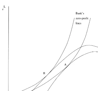
An example of this counter-intuitive result is shown in Figure 3. The original equilib-rium is at pointA. An increase inh, by reducing the bank’s return on its reserves, raises its zero-profit curve. The new equilibrium point is atB. As shown in the diagram, it is
9Gray and Wu (1995) also find that higher costs of funds for lenders can lower the loan interest rate. In their
possible for the new loan rate to be below the old. Implicit differentiation of equation (4) yields:
dr#L
dr# 5
1
P~I*!
S
12e~r#!
h~r#!
D
(15)where,
e~r!5P9~I*~r!! P~I*~r!! I*~r!)
and
h~r!5R0~I*~r!! R9~I*~r!!I*~r!
Given our assumptions aboutP(I)andR(I), botheandhare negative. As a result, the sign of the derivative in equation (15) is ambiguous. If h is small (in absolute value) relative toe, then r#Lcould rise as a result of an increase inr#. Note thathis the inverse
of the elasticity of I* with respect to 1 1 r, and sor#L is more likely to decline if an increase inrcauses a large decline in the size of loans and so a relatively large reduction in the probability of default. Note, however, that even in this case the expected return on loans,r, would rise. The perverse result forr#Lis due only to a change in the riskiness of loans.
The increase in the rate of growth of high-powered money causes an increase in investment. The higher “inflation tax” on deposits reduces the level of deposits, and thereby the demand for high-powered money. The decline in H# raises aggregate invest-ment. Thus, there is a Tobin effect in the model. Note, however, that the investment is less efficient because the tax wedge between the borrowing and lending interest rates has been increased. In Section IV, I show that the optimal steady-state rate of growth of the money supply is zero. (This result is intuitive because it amounts to removing a distortionary tax.)
Change in the Required Reserve Ratio
An increase inf, the required reserve ratio, forces banks to hold a larger portion of their assets as non-interest-bearing reserves. Thus, the increase causes a rise in the banks’ cost of funds,r, for a givenrD. Because of the increase inr, borrowers choose smaller loans than before the policy change. On the other hand, the increase infincreases the amount of deposits required to fund a loan of a given size because a smaller portion of deposited funds can be loaned out owing to the higher reserve requirement. Thus, banks’ demand for funds from depositors could rise or fall. As in the case of a rise inh, there is no effect on the supply of funds to banks,D(rD). As a result, the effect onr
#D, and therefore onD(r#D), is ambiguous. One can show that:
dr#D BecauseL9(r) is negative, the final fraction on the right-hand side of (16) is positive. However, ifL9(r) is large in absolute value or the difference between the expected return on loans, 11r#, and that on reserves, (11 n)/(11h), is large, then the term in square brackets could be negative and a rise infwould cause a decline in the deposit interest rate. In this case, the increase inr#generated by the rise infcauses a large decline in loan demand. As a result, banks’ demand for deposits falls, and the deposit rate falls. In contrast, ifL9(r) is small or the difference between the returns on loans and reserves is small, then loan demand does not change much in response to the rise inr#. In this case, the demand for deposited funds rises, and so the deposit rate is driven up. As in the case of an increase in h, the banks’ return on loans must rise, butr#Lneed not do so.
One would expect that an increase in f would raise the demand for reserves, and thereby reduce aggregate investment. This need not be the case, however. The effect on aggregate investment is given by:
such a case, aggregate investment would rise. As in the case of an increase inh, however, investment would become more inefficient because of the larger tax wedge.
Change in the Level of Government Debt
An increase inB, the level of government debt per member of the young cohort, does not affectrfor a given value ofrD, and so it has no effect on the aggregate demand for loans. It also has no effect on individuals’ holdings of financial assets. Thus, the only effect of an increase inBis the direct increase in the demand for funds caused by the increase in government borrowing. The effect of this change is clearly to raiser#DandD(r#D). The rise inr#Dinduced by this change raisesr#and so reduces the size of loans. As in the two cases above, the effect of this change onr#Lis not clear.
Not surprisingly, the increase in government debt crowds out investment. The effect on investment is given by:
dI#
dB52~12f!2fD9~r#
D! dr# D
dB (18)
The first term in this expression is the direct effect of the increase in government borrowing. Note that this effect is less than one-for-one because some of the funds the government borrows would have been held as reserves by the banking sector in any case. The second term takes account of the effect the increase inr#Dhas on the level of financial asset holding. By increasing r#D, the policy change raises the level of financial assets people hold, and thereby raises the level of reserves. Both terms are negative, and the effect on investment is therefore negative.
The Effects of Rationing
These results are quite similar to those found in models without rationing such as Romer (1986). The main difference here is that the loan interest rate may not rise as expected when lending is cut back. Thus, if the monetary authority focuses attention on the loan interest rate as a measure of how tight monetary policy is, it may be deceived. However, the possible perverse movements in the loan interest rate reflect shifts in the risk premium on loans rather than in the expected return on loans. So long as the monetary authorities restrict their attention to the risk-free rate on government bonds or deposits (or to the expected return on loans,r) interest rate movements would be as one would expect from models without rationing.
IV. Welfare Effects
In this section, I consider the problem of a central planner attempting to maximize social welfare, derive the set of policies that maximize steady-state welfare, and analyze the effects of rationing under welfare-maximizing policies.
Optimal Policy
If the planner assumes that all individuals have identical linear utility functions, then this problem is equivalent to maximizing expected aggregate consumption. If the planner refunds government revenues to each period’s old generation, then steady-state consump-tion per member of the old cohort is:
C# 5~11r#D!D~r#D!1R~I#**!
E
The first term in this expression is the second-period return on the financial assets of the old generation. The second, third, and fourth terms are the returns on investment, less expected loan repayments (if any), of those with high, medium, and low endowments respectively. The final term is the level of government revenues per member of the old cohort. By substituting the balance sheet identity of the banking sector into this expres-sion, The central planner’s problem can be expressed as:
@~11n!f 2~11#rD!#D9~r#D! dr#
D
dh 1~11r#!L9~r#! dr#
dh50 (21)
@~11n!f 2~11#rD!#D9~r#D! dr# D
dB 1~11n!12f)50 (22) Using comparative statics on equation (9) and equation (10) to evaluate the derivatives in these expressions, one can show that an optimal policy implies:10
1
11p# 511n,i.e., h50 (23)
r#5r#D5n (24)
P~I#*~n!!~11r#L!511n (25)
In fact, there is a continuum of optimal policies for the economy. As indicated in equation (23), the government should set hequal to zero. Doing so eliminates the tax wedge between the borrowing and lending interest rates by equating the return on high-powered money to the return on loans and deposits.11The government should then choosefandBso as to equate the marginal return on investment to the rate of population growth, as shown in equation (24). This is simply the dynamic efficiency result of Diamond (1965). For an arbitraryB[Bless thanD(n)2L(n)], the optimalfis given by:
f 512 L~n!
D~n!2B (26)
The final condition, equation (25), shows that the optimal loan interest rate is greater than n because of the probability of default.
Of course, there may not be an interior maximum for the government’s problem. In particular, if the government choosesfequal to zero to eliminate the tax wedge, and sets B equal to zero, then it could still be the case that the marginal return on storage is greater than the rate of growth of the population. In this case, the government could raise steady-state welfare by lending to the country’s citizens—i.e., choosing a negative level of government debt.
To implement such a policy, the government would have to tax the endowment of the initial old generation. It would take resources from the initial old and deposit them at banks (or alternatively, make direct loans itself). The amount taken from the initial old would have to be chosen to drive the marginal expected return on projects to the rate of growth of the population. Thus, the repayments on the loans would just supply the funds to loan to the next generation, and so the policy could be continued.
This result is similar to Smith’s (1983) “optimal government lending policy.” Smith considers an endowment economy in which there is a rationing equilibrium similar to this one. The model has no required reserves (although agents choose to hold money in
10Because the results are intuitive and the proof provides no additional insight, it is not provided here. An
unpublished appendix to the paper containing a proof is available from the author on request.
11This is just the Friedman rule—choose the rate of growth of the money supply to equate the return on
equilibrium). In the model the government can raise steady-state welfare by taxing the initial old, and using the proceeds to make additional loans to the borrowers. So long as the expected repayments on the loans are greater than or equal to the amount loaned, the government can feasiblely implement such a policy. Implementing the policy will clearly raise welfare of borrowers, and Smith shows that there are taxes and transfers which make all agents (other than the initial old) better off.
One should note, however, that this result can arise in models without rationing. For example, one would obtain a similar result in a model like that of Diamond (1965), in which the economy is dynamically efficient. In that model, the government could also take some of the capital of the old generation, and use it to make loans to the young. By so doing, the government could drive the marginal product of capital closer to the rate of growth of the population, and raise the consumption of every generation but the initial old.
The Welfare Implications of Rationing
If the level of borrowing were not observable, then the rationed equilibrium would not be attainable [see Kletzer (1984)]. What would be the welfare implications of not having the rationing?12The first-order condition for the agents’ optimal unconstrained choice of loan
size given an interest rate, rLwas derived earlier:
R9~w1L!2P~w1L!~11rL!2P9~w1L!~11rL!L50 One can rewrite this as:
R9~w1L!5~11r!
S
11e Lw1L
D
(27)where, as defined above:
e~r!5P9~I*~r!! P~I*~r!! I*~r!
andeis less than zero. Thus, for a given value ofr, borrowers will borrow too much, setting the expected marginal product of storage belowr.13 As noted above, efficiency requires that all borrowers have the same project size, with the marginal expected return on investment equal to the rate of population growth. If the government is restricted to choosingh,f, and B, then this condition cannot be met in an unrationed equilibrium. If all borrowers had the same project size, thenR9(w1L)would be the same for all, ande would be the same for all. Thus, the condition in equation (27) could not hold for all borrowers becauseL/(w1 L)would vary inversely with the borrowers’ endowments.
Thus, so long as government policy is optimal, rationing raises welfare in this model. This result is not a surprise. As in de Miza and Webb (1992), the rationing comes from allowing contracts to specify both the interest rate and the amount borrowed. Because
12I consider here the outcome if the underlying storage technology remains the same. If the probability of
default were fixed, independent of the amount invested, then there would be no need for rationing. In that case, one would need to assume thatrˆis decreasing inIin order to have decreasing returns to scale in storage. Such a model would be almost identical to the “pure banking economy” considered in Romer (1985).
13Of course, in equilibrium this increase in demand will driverhigher. The resulting level of intermediation
there is no information problem in the model, the rationed lending contract is first best. Thus, if the amount borrowed were private information, we should expect the equilibrium to be less efficient.
V. A More Complex Financial Structure
One problem with the model presented thus far is that the banks would be dominated by a bond market, because by using bonds to lend among themselves, agents could avoid the tax that required reserves impose on intermediation. In this section I relax the assumption, which I have maintained until now, that direct loans between agents are not possible.
There are three possible ways to add a bond market to the model without completely eliminating the banking sector. First, one can assume that banks are useful for some, but not all borrowers, because they provide screening or monitoring services more efficiently than decentralized lenders could [Diamond (1984)]. Second, one can impose that the two types of credit have different cost structures. For example, if there were a substantial fixed cost of using the bond market, perhaps to provide information in a form acceptable to market participants, then those who want to borrow small amounts would choose to borrow from a bank, even if in doing so they incur a proportional tax. Finally, following Romer (1985), one could assume that deposits provide transactions or other services. In this case, banks need not pay a return on deposits that is competitive with the return on private loans. As Fama (1985) points out, however, the rate paid on certificates of deposit— banks’ marginal source of funds—is virtually identical to that paid on commer-cial paper. Thus, borrowers from banks, not depositors, appear to bear the incidence of the tax.
In this section I consider the effect of adding a bond market with a fixed entry cost–the second strategy just mentioned—to the model presented earlier. In particular, I allow borrowers to borrow directly from other individuals in a bond market by paying a fixed cost ofk. I assume that thekunits can be borrowed if the individual’s endowment is less thank.
The Individuals’ Problem
A potential borrower faces a more complex problem in this case. It is:
Maximize: L,BC
R~w1L1BC2jBk!2~11r!L2~11rBC!BC
where L is the size of the bank loan,BC is the amount of credit obtained in the bond market,jBis one if the bond market is used and zero if it is not, andrBCis the expected return investors demand on private bonds. Because investors are risk neutral, the expected return on private bonds must equal that on government debt or bank deposits in equilib-rium:
r#BC5r#B5r#D (28)
second period income. Thus, individuals will choose the better of the following alterna-tives:
L5I*~r!2w,BC50 or,
BC5I**~rD!2w1k,L50
Notice that in each case the marginal expected return on investment equals the cost of funds.
For large enough values ofk, no individual will ever choose to use the bond market, regardless of endowment size. Conversely, for small values ofk, bank credit will never be chosen. I focus here on values of k that lead to both forms of credit being used in equilibrium, depending on the borrower’s endowment size. As one would expect, those individuals with small endowments find it worthwhile to pay the entrance fee and get the lower bond market interest rate on a large loan, while those with larger endowments borrow a smaller amount at the higher interest rates charged by banks. I definew* to be the endowment size at which agents are just indifferent between the two alternatives. Thus, atw*:
R~I*~r!!2~11r!~I*~r!2w*!5R~I**~rD!!2~11rD!~I**~rD!2w*1k! where I have substitutedrDfor rBC . Solving forw* yields:
w*~r, rD!5 1
r 2rD@R~I**~rD!!2R~I*~r!!
2~11rD!~I**~rD!1k!1~11r!I*~r!# (29) Note thatw* is decreasing inrDand increasing in r, because a higher rDmakes it less worthwhile to pay the cost of borrowing in the bond market, while a higherr makes it more worthwhile to do so.
The demands for credit from bond market borrowers and from banks (per member of the young cohort) are given by:
BC~r,rD!5
E
0
w*~r,rD!
~I**~rD!2w1k!f~w!dw (30)
and,
L~r,rD!5
E
w*~r,rD!I*~r!
~I*~r!2w!f~w!dw (31)
Steady-State Conditions
In the new model, the amount of deposits at banks equals the total financial assets of individuals, D, less their holdings of private and government bonds (BC 1 B). Thus, market clearing in the funds and money markets are given by:
D~r#D!5 1
12f L~r#,r#
D!1BC~r#,r#D!1B (32)
and,
H# 5f~D~r#D!2BC~r#, r#D!2B! (33) The left-hand side of equation (32) is the supply of savings, and the right-hand side is the demand for savings. As before, the 1/(12 f) term accounts for the fact that it takes 1/(12f) dollars of deposits to fund a dollar of loans, henceL(r,rD)/(12f) is the indirect demand for funds by bank borrowers. By substituting the expression forrfrom equation (10) into equation (32), one can again solve for the steady-state value ofrD.14 Finally,
there is now a third interest rate,rBC, which is the interest rate on private loans. In order for agents to be willing to make these loans, it must be the case that:
P~I**~r#D!!~11r#BC!511r#D (34) The other steady-state conditions for the economy remain unchanged.
Effects of Changes in Policy Variables
The effect of a change in the level of government debt,B, on the deposit interest rate is the same as before. As in the simpler model, the demand for funds rises for each level of rD, while supply remains the same. Thus,r#Drises, holdings of financial assets by savers increase, and the private demand for funds decreases.
The effect of increased government borrowing on the level of investment is less clear, however. In the more complex model, the level of investment is given by:
I#5w# 2k#2~12f!B2f@D~r#D!2BC~r#,r#D!# (35) wherek# is the per capita cost of using the bond market:
k#5k
E
0
w*
f~w!dw (36)
One can show that the change in the level of investment owing to an increase inBis:
14One can show that the aggregate demand for funds is still a decreasing function ofrDin this more complex
dI#
As in the simple model, the first two terms are negative. The third term takes account of the fact that an increase inrDinfluences the decision to borrow either through banks or directly in the bond market. Its sign is ambiguous because the relative sizes of the two partial derivatives are not known. If the increase in the deposit rate causes a net shift of borrowing from banks to the bond market, then demand for reserves will decrease, boosting investment. On the other hand, the higher deposit rate could cause credit demand to shift in the other direction, increasing holdings of reserves and trimming investment. The final term captures the change in the costs of accessing the bond market. Its sign is also ambiguous, but in many cases will be the reverse of the third term. (If the higherr#D
causes a shift toward bond issuance, holdings of reserves will fall but bond market entry costs will rise.) So long asfandkare not too large, the first term will dominate and an increase in government debt will crowd out investment.
The effects of a change in the rate of growth of high-powered money,h, on interest rates are ambiguous in the more complicated model. An increase in h raises the steady-state inflation rate which raisesrfor a given level ofrD. This change has two effects. First, the rise in rreduces loan demand by those borrowing from banks, thereby reducing the demand for funds. Second, the increase in r causes a rise in BC, thereby boosting the demand for funds, as some individuals who were using banks now find the bond market preferable. The net effect of the rise inhonrDdepends on which of these effects is larger. Because the impact of an increase in h on interest rates is unclear, its effect on investment is also ambiguous. One can show that:
dI#
The first term again captures the effect of the change in holdings of financial assets on reserves demand; it is negative as long as the increase inhdecreasesr#D. The second term takes account of the fact that the increased inflation tax affects the borrower’s decision to issue bonds or obtain bank loans, whereas the final term takes account of changes in the number of individuals borrowing directly in the bond market, and the resulting effect on the amount of resources used to buy access to the market. The signs of these two terms are ambiguous.
As in the simpler model, the effects of an increase infare uncertain.
In spite of the more complex financial structure, the welfare results from Section III also still hold here. Note that if the government eliminates the tax wedge between borrowing and lending, then all loans will be made through banks. This is reasonable because it allows the society to avoid the deadweight loss of the cost of borrowing through the bond market.
VI. Concluding Remarks
In this paper I have shown that the effects of policy in a model with a particular type of endogenous credit rationing are quite similar to those in a model without rationing. This result suggests that it need not be true, as Stiglitz claims, that in models with credit rationing, “Monetary policy . . . has effects not through the rate of interest (variations in real rates of interest until recently have been too small to account for much of the variability in investment or savings), but through its effects on the supply of credit” (Stiglitz, 1987, p. 38). In the credit rationing model presented here the marginal return on borrower’s projects is always equal to the bank’s cost of funds. Government policies work because they change that cost, not because they have a direct effect on quantities.
The source of the confusion is that, as in Figure 3 above, the loan interest rate may not rise when there is a contraction in lending. In fact, Stiglitz (1987) has a figure much like Figure 3 (Figure 10b, p. 12), and claims that, “an increase in the supply of credit available may have no effect on interest rates, but may simply lead to more loans (less credit rationing) at the old interest rates.” As the model in this paper makes clear, however, in such cases the banks’ cost of funds is falling, and borrowers are increasing their loan sizes in response. In the new equilibrium, the expected rate of return on loans will be lower than before the change.
A natural response to the model presented in this paper is to claim that it is too simple. There is no incentive problem, for example, and no adverse selection problem. It is clear, however, that the addition of these complications need not affect many of the results found here. For example, one could consider the policy implications of a rationing model like that in Keeton (1979). Keeton assumes that larger loans are riskier, not because of the technology, but because highly leveraged borrowers have an incentive to choose riskier projects. In such a model the equilibrium looks very similar to the equilibrium presented here. There is an upward sloping–perhaps even backward-bending—zero-profit line for the banks. Borrowers still choose their favorite point on the zero-profit line.
Putting such a model into the general equilibrium framework employed in this paper would make the results more complex. In particular, the equilibrium project size would be a function of the agent’s endowment size. Nonetheless, if there were a reduction in the supply of funds in such a model–resulting, for example, from an increase in the level of government debt–the banks’ zero-profit line for each borrower would shift up and to the left. As a result, the level of borrowing would fall and the expected return on loans would rise. Thus, the increase in government debt would act on the economy along familiar lines, and not through any direct quantity mechanism. Moreover, depending on the details of the model, perverse movements in the loan interest rate could be possible.
Such a change in the model could affect the welfare results reported in this paper because the rationed lending contract would likely no longer be first best. As a result, optimal government policy could be more complex.
others not obtaining loans.15 As noted in Keeton (1979), this sort of rationing arises if there is a loan size and loan interest rate that maximize the banks’ return on loans. [See also the discussion in Stiglitz and Weiss (1981), p. 408]. If such an optimal loan size and interest rate exist, and if banks’ cost of funds in equilibrium is driven to this maximal level, then in the equilibrium some borrowers will obtain loans of the optimal size at the optimal interest rate while other identical borrowers will not. With rationing of this type, credit market policies could have direct effects on the quantity of credit supplied without affecting either the expected return on loans or the deposit interest rate.16Thus, the claims in Blinder and Stiglitz (1983) and elsewhere about the implications of rationing for the impact of monetary policy would be true in such a model. Indeed, such a model may be what these authors had in mind (although the figure and discussion in Stiglitz (1987) suggest that a distinction between the effects of different types of credit constraints was not being clearly made).
In short, the terms “credit rationing” and “credit constraints” are too broad. Different models of credit constraints have different implications both for Ricardian Equivalence (as in Hayashi, 1987), and for monetary policy. Moreover, models can have interesting implications for one issue, and quite ordinary implications for the other. For example, consider a model in which one group of agents is subject to severe incentive problems and so cannot obtain credit at any rate, while remaining agents never default. In such a model monetary policy would have quite ordinary effects, but the economy would not be Ricardian.
References
Blinder, A.S., and Stiglitz, J.E. 1983. Money, credit constraints, and economic activity.American Economic Review73(2):297–302.
Clark, P.K. 1979. Investment in the 1970s: Theory, performance, prediction.Brookings Papers on Economic Activity73–113.
Clark, P.K. 1993. Tax incentives and equipment investment. Brookings Papers on Economic Activity317–347.
de Miza, D., and Webb, D.C. 1992. Efficient credit rationing.European Economic Review36(6): 1277–1290.
Diamond, D. 1984. Financial intermediation and delegated monitoring.Review of Economic Studies
51(3):393–414.
Diamond, P.A. 1965. National debt in a neoclassical growth model.American Economic Review
55(5):1126–1150.
Fama, E.F. January 1985. What’s different about banks?Journal of Monetary Economics15:29–40. Fazzari, S.M., Hubbard, R.G., and Peterson, B.C. 1988. Financing constraints and corporate
investment.Brookings Papers on Economic Activity141–195.
15Keeton (1979) refers to such an outcome as “type II” rationing, whereas Stiglitz and Weiss (1987) refer
to it as “criterion a” rationing.
16Fuerst (1994) presents such a model. His model includes increasing returns to scale in monitoring costs
Fuerst, T.S. 1994. The availability doctrine.Journal of Monetary Economics34(3):429–443. Gray, J-A., and Wu, Y. Summer 1995. On equilibrium credit rationing and interest rates.Journal
of Macroeconomics17(3):405–420.
Hall, R.E., and Mishkin, F. 1982. The sensitivity of consumption to transitory income: estimates from panel data on households.Econometrica50:461–481.
Hayashi, F. 1987. Tests for liquidity constraints: A critical survey and some new observations. In
Advances in Econometrics, Fifth World Congress (T.F. Bewley, ed.). London: Cambridge University Press, Chap. 13.
Hubbard, R.G., Kashyap, A.K., and Whited, T.M. 1995. Internal finance and firm investment.
Journal of Money, Credit and Banking27(3):683–701.
Jaffee, D., and Stiglitz, J. 1990. Credit rationing. In Handbook of Monetary Economics, Vol. II (B.M. Freidman, and F.H. Hahn, eds.). New York: North Holland.
Kashyap, A.K., and Stein, J.C. 1994. Monetary policy and bank lending. InMonetary Policy(N.G. Mankiw, ed.). Chicago: University of Chicago Press.
Keeton, W. 1979.Equilibrium Credit Rationing. New York: Garland Press.
Kletzer, Kenneth. 1984. Asymmetries of information and LDC borrowing with sovereign risk.
Economic Journal94(2):287–307.
Poterba, J.M., and Summers, L.H. 1987. Finite lifetimes and the effects of budget deficits on national saving.Journal of Monetary Economics20(2):411–436.
Riley, J.G. 1987. Credit rationing: A further remark.American Economic Review77(1):224–227 Romer, D. 1985. Financial intermediation, reserve requirements, and inside money: A general
equilibrium analysis.Journal of Monetary Economics16(2):175–194.
Roosa, R.V. 1951.Money, Trade and Economic Growth, in Honor of John H. Williams. New York: Macmillan.
Smith, B. 1983. Limited information, credit rationing, and optimal government lending policy.
American Economic Review73(3):305–318.
Stiglitz, J.E. 1987. The causes and consequences of the dependence of quality on price.Journal of Economic Literature25(1):1–48.
Stiglitz, J.E., and Weiss, A. 1981. Credit rationing in markets with imperfect information.American Economic Review71(1):393–410.
Stiglitz, J.E., and Weiss, A. 1987. Credit rationing: Reply.American Economic Review77(1):228– 231.
![Figure 2. Equilibrium in the market for funds [Equation (9)].](https://thumb-ap.123doks.com/thumbv2/123dok/3102284.1376170/10.612.99.444.57.343/figure-equilibrium-market-funds-equation.webp)