On the double points of a Mathieu equation
P.N. Shivakumara;∗;1, Jungong Xueb;2
aDepartment of Mathematics, Institute of Industrial Mathematical Sciences (IIMS), University of Manitoba,
Winnipeg, Manitoba, Canada R3T 2N2
bDepartment of Mathematics, Fudan University, Shanghai, 200433, People’s Republic of China
Received 6 October 1998
Abstract
For a Mathieu equation with parameterq, the eigenvalues can be regarded as functions of the variableq. Our aim is to nd qwhen adjacent eigenvalues of the same type become equal yielding double points of the given Mathieu equation. The problem reduces to an equivalent eigenvalue problem of the formBX=X;whereBis an innite tridiagonal matrix. A method is developed to locate the rst double eigenvalue to any required degree of accuracy when qis an imaginary number. Computational results are given to illustrate the theory for the rst double eigenvalue. Numerical results are given for some subsequent double points. c1999 Elsevier Science B.V. All rights reserved.
Keywords:Mathieu equation; Double point; Diagonally dominant matrix; Innite tridiagonal matrix
1. Introduction
The motivation for this work comes from the discussion of eigenvalues for the Mathieu equation d2y
dx2 + (−2qcos 2x)y= 0: (1.1)
∗Corresponding author. Tel.: 204-474-6724; fax: 204-474-7602.
E-mail address: [email protected] (P.N. Shivakumar).
1
Supported in part by the National Sciences and Engineering Research Council of Canada under grant A7899 and by the Visitors Program of IIMS.
2This work was completed when the author visited IIMS of the University of Manitoba under its Visitors Program
during the summer of 1998. Partial travel support was provided by the National Science Foundation of China.
In general, Mathieu equations do not have periodic solutions (see [3]). If q is a real number, there exist innitely many distinct eigenvaluescorresponding to periodic solutions. For a detailed account of eigenvalues of (1.1) when q is real see [6].
Our interest is in the case when two consecutive eigenvalues merge and become equal for some values of parameter q. This pair of merging points is called a double point of (1.1) for that value of q. In this paper, we will discuss only real double points. It has been studied in [1] that for real double points to occur, the parameter q must attain some pure imaginary value. A comprehensive account of the eigenvalues of (1.1) and its branch points are given in [4]. They give an account of asymptotic expansions for eigenvalues. Blanch and Clemm [2] use truncated power series expansions for the eigenvalues and evaluate approximate values for q when it results in a double eigenvalue. Their result, while giving excellent numerical values for a number of particular cases, does not have a computable error analysis. There does not seem to be any earlier results concerning double points which include an error analysis. For nite matrices, Lippert and Edelman [5] develop heuristical and geometrical techniques to locate double eigenvalues. In this paper, we shall develop an algorithm to compute some special double points. Theoretically, this method can achieve any required accuracy. For these special double points, the numerical results compare very well with that of Blanch and Clemm.
Throughout the paper we concentrate on the solution of (1.1) with the boundary conditions
y(0) =y(=2) = 0:
Using an even solution of the form
y(x) =
∞ X
r=1
xrq−rsin 2r x;
equation (1.1) yields the innite linear algebraic system
BX=X; (1.2)
where B is an innite tridiagonal matrix B= (bij) given by
bij=
−Q; j=i−1; i¿2;
4i2; j=i;
1; j=i+ 1; i¿1:
Here Q=−q2¿0 and X = (x
1; x2; : : :)T: This means is an eigenvalue of the innite matrix B.
2. Notations and preliminaries
We use the notation Ak; n to denote the principle submatrix ofA=B−I from the kth row to the
nth row, i.e.,
Ak; n=
4k2− 1
−Q 4(k+ 1)2− 1
−Q 4(k+ 2)2− 1
. .. . .. . ..
−Q 4n2−
: (2.1)
We dene
ak; n=ak; n(; Q) = detAk; n; dk; n= n
Y
j=k
4j2
and
fk; n=fk; n(; Q) =ak; n(; Q)=dk; n;
where ak; k−1=an+1; n= 1.
First we give an expansion formula for ak; n:
Lemma 2.1. If k6l6n−1;then
ak; n=ak;lal+1; n+Qak;l−1al+2; n: (2.2)
Proof. Expanding the determinant ak; n along the rst row, we get
ak; n=ak; kak+1; n+Qak+2; n:
Clearly (2.2) holds when l=k: Assuming that (2.2) holds for l=j6n−2 and expanding the determinant aj+1; n along the rst column, we obtain
ak; n=ak; jaj+1; n+Qak; j−1aj+2; n
=ak; j(aj+1; j+1aj+2; n+Qaj+3; n) +Qak; j−1aj+2; n
=aj+2; n(ak; jaj+1; j+1+Qak; j−1) +Qak; jaj+3; n
=ak; j+1aj+2; n+Qak; jaj+3; n:
Hence, Eq. (2.2) holds for l=j+ 1; which completes the proof.
It follows from (2.2) that
fk; n=fk;lfl+1; n+
Q
16l2(l+ 1)2fk;l−1fl+2; n: (2.3)
Also it is easy to show by induction that if 4k2− ¿0 and Q ¿0, then
0¡ ak; j6ak+1; j+1 and
ak;lal+2; j
ak; j
6 1
4(l+ 1)2−; j¿k:
Lemma 2.2. If 4k2− ¿0 andQ ¿0;then
0¡@ak; n
@Q ¡ g(; k+ 1)ak+1; n; (2.4)
0¡−@ak; n
@ ¡ g(; k)ak; n; (2.5)
whereg(; k) =P∞
j=k 1 4j2−:
Proof. With ak; k−1= 1 and an+1; n= 1; we have
@ak; n
@Q =
n−2
X
j=k−1
ak; jaj+3; n
6
n−2
X
j=k−1
ak+1; j+1aj+3; n
6
n−2
X
j=k−1
ak+1; n
4(j+ 2)2−1
¡ g(; k+ 1)ak+1; n:
Similarly,
−@ak; n
@ =
n−1
X
j=k−1
ak; jaj+2; n6ak; n n−1
X
j=k−1
1
4(j+ 1)2−¡ g(; k)ak; n:
On using (2.4) and (2.5), we can bound second partial derivatives of ak; n: We get
@2a k; n
@Q2 = n−2
X
j=k−1
@a
k; j
@Q aj+3; n+ak; j @aj+3; n
@Q
6
n−2
X
j=k−1
(g(; k+ 1)ak+1; jaj+3; n+g(; j+ 4)ak; jaj+4; n)
62g(; k+ 1)
n−2
X
j=k−1
ak+1; j+1aj+3; n
¡2g(; k+ 1)2ak+1; n: (2.6)
Similarly we can show that
0¡@
2a k; n
@2 ¡2g(; k) 2a
k; n (2.7)
and
0¡−@
2a k; n
@@Q¡2g(; k)g(; k+ 1)ak; n: (2.8)
We will now prove that as n tends to ∞; fk; n converges uniformly in each bounded and closed
Lemma 2.3. Let be a bounded and closed region in (:Q)∈(−∞;+∞)×(0;+∞:) For eachk
the jth eigenvalue of Ak; n lies in the interval
[4(k+j−1)2−−Q−1;4(k+j−1)2−+Q+ 1]: to show that fk; n also converges uniformly.
Dening
fk= lim n→∞ fk; n;
it is clear that fk is continuous in (; Q)∈(−∞;+∞)×(0;+∞):Using the method of proof Lemma
3, we can prove that the partial derivatives
3. The rst double point
Since f(; Q)¿0 if ¡4 and Q ¿0; the real double points lies in the interval [4;∞); which we partition into seperate sub-intervals
[0;∞) =
∞ [
k=1
Ik;
where Ik= [4k2;4(k+ 1)2):
In this section, we will prove that there exists a unique double point in the interval [4;16]. In other words, we prove that there is only one solution to Eq. (2.9).
Lemma 3.1. If ∈[4;16] and a1;2=Q+ (−4)(−16)¿0; then
@f1
@Q ¿0:
Proof. Noting that
g(;5) =
∞ X
j=5
1 4j2−6
∞ X
j=5
1 4j(j−1)6
1 16
and
a1; n=a1;2a3; n+Qa1;1a4; n;
we have
@f1
@Q = limn→∞
1
d1; n
·@a1; n
@Q
= lim
n→∞
1
d1; n
@a
1;2
@Q a3; n+a1;2 @a3; n
@Q +a1;1a4; n+Qa1;1 @a4; n
@Q
¿ lim
n→∞
1
d1; n
a3; n+ (4−)a4; n+
4−
16 Qa5; n
= lim
n→∞
1
d1; n
2(20−)a4; n+
Q(20−) 16 a5; n
¿ lim
n→∞
8a4; n
d1; n
¿0:
Choosing k= 1 and letting n→ ∞ in (2.3) yields
f1=f1; lfl+1+
Q
16l2(l+ 1)2f1; l−1fl+2; (3.1)
from which we can establish
Lemma 3.2. IfQ ¿0andf1; l−1f1; l¿0;thenf1¡0iff1; l−1¡0or f1; l¡0;andf1¿0iff1; l−1¿0
Proof. Since
f1; j=f1; j−1fj; j+
Q
16j2(j−1)2f1; j−2 for j6l;
by induction we can show that sign(f1; j) = (−1)j for ¿4l2: From f1; l−1f1; l¿0; we have 64l2;
which means fk¿0 for k¿l+ 1: Using (3.2) completes the proof.
If ∈(4;16); f1;1¡0:Consequently, if f1;260; i.e., Q6(−4)(16−); then f1¡0: If f1;3¿0,
then f1;2¿0; f1¿0 and
Q ¡(36−)(16−)(−4)
2(20−) :
Since f1 is a continuous function, from Lemma 3.2 there exists a unique Q for each such that
f(; Q) = 0. We regard this Q as a function of and write it as Q=Q(). Obviously,
(−4)(16−)6Q()6(36−)(16−)(−4)
2(20−) : (3.2)
Using Lemma 3.1 and Dierentiating f1(; Q) = 0 with respect to , we have
Q′
() =−@f1=@
@f1=@Q
: (3.3)
Because Q(4) =Q(16) = 0; there exists at least one point 0 in interval [4;16] such that Q′(0) = 0;
i.e., @f1=@|(0; Q(0)) = 0; which means that 0 is a double point and Q(0) is the corresponding
singular point.
Now we show that there is a unique double point in [4;16]. To do this, we rst need the following lemma.
Lemma 3.3. If is a double point in [4;16]; then
¡55
4 :
Proof. From
f1=
4−
4 f2+
Q
64f3= 0;
f2
f3
= 1 16 ·
Q
(−4): (3.4)
We can easily check that g(;3)62=15 and g(;4)61=12: Thus
−@f3
@ = limn→∞
1
d3; n
−@a3; n
@
¡ g(;3)· lim
n→∞ a3; n
d3; n
6 2
15f3 and
−@f4
@6
We have
Combining (3.4) and (3.5) produces
Q()¿15(−4)
2
2+ 7 :
Using the right inequality of (3.2), we have the inequality (2+ 7)(36−)(16−)
30(20−)(−4) ¿1;
which can easily be shown that it does not hold if ¿55 4.
Using Lemma 3.3, we prove the following
Lemma 3.4. If is a double point in [4;16]; then Q′′
()¡0:
Proof. Dierentiating (3.3) gives
Q′′
the problem reduces to establishing that @2f
we can write
@2f 1
@2 =
@2f 1;2
@2 f3+ 2
@f12
@ · @f3
@ +f12 @2f
3
@2 +
Q
576 −2
@f4
@ +
(4−)@2f 4
@2
!
¿ f3
32 +
−10 16 ·
@f3
@ +
Q
576
2−4−
6 −
@f4
@
¿ f3
32
1−4|−10|
15
f3¿0;
which completes the proof.
Now we present the main result of this section.
Theorem 3.1. There exists a unique double point in [4;16].
Proof. We only need to prove uniqueness. If there are two double points 0¡ 1 in [4;16], from
Lemma 7, Q′′(
0)¡0; Q′′(1)¡0: Without loss of generality, we assume that there are no other
double points in (0; 1); which means that Q′() remains positive or negative. We assume it is
positive. Then, Q′(
0)¿0; which contradicts with Q′(0)¡0:
In Section 5, we will present an algorithm to compute this double point in [4;16].
4. The interval [16;36]
In this section, we will prove that there are no double points in the interval [16;36]. To do this, it suces to show that if ∈[16;36] and Q ¿0 satisfying f1(; Q) = 0; then
@f1
@
(; Q)
¡0:
First we need to bound Q in terms of . Since
0 =f1=f1;3f4+
Q
16·32·42f1;2f5
and f1;2; f4; f5 are all positive,
f1;3¡0;
which implies that
(36−)[(−4)(−16) +Q] + (4−)Q ¡0:
It follows that ¿20,
Q¿(36−)(−4)(−16)
2(−20) (4.1)
and
On the other hand,
f4
f5
= 1 4·42
(64−) + Q 4·52 ·
f6
f5
6 1
4·42
64−+ Q 100−
yields
Q=−16·3
2·42f 1;3f4
f1;2f5
6 (−4)Q
(−4)(−16) +Q
64−+ Q 100−
;
which on simplication gives
Q6(−4)(40−)(100−)
52− : (4.2)
Lemma 4.1. Let ∈[16;36] and Q ¿0 satisfying f1(; Q) = 0; then for k¿4
a1;3a4; k +Qa1;2a5; k= (−Q)k
−3a 1;3 lim
n→∞ ak+2; n
a5; n
: (4.3)
Proof. Letting a5;3= 0; we have
a1; n=a1;3a4; n+Qa1;2a5; n
=a1;3[a4; kak+1; n+Qa4; k−1ak+2; n] +Qa1;2[a5; kak+1; n+Qa5; k−1ak+2; n]
= (a1;3a4; k+Qa1;2a5; k)ak+1; n+Q(a1;3a4; k−1+Qa1;2a5; k−1)ak+2; n:
Since
f1= lim n→∞
a1; n
d1; n
= 0;
a1;3a4; k +Qa1;2a5; k=−Q(a1;3a4; k−1+Qa1;2a5; k−1) lim n→∞
ak+2; n
ak+1; n
= (−Q)k−3(a
1;3a4;3+Qa1;2a5;3) lim n→∞
ak+2; n
a5; n
= (−Q)k−3a 1;3 lim
n→∞ ak+2; n
a5; n
:
Because a1;3¡0, we can conclude that a1;3a4; k+Qa1;2a5; k is positive if k is even and negative if
k is odd. To prove the main result of this section, we still need the following lemma.
Lemma 4.2. Let ∈[16;36] and Q ¿0 satisfying f1(; Q) = 0. Then
0¿−a1;3
@a4; n
@ −Qa1;2 @a5; n
@ ¿
121
Proof. From Lemma 4.1,
The following theorem is the main result of this section.
Theorem 4.1. There are no double points in [16;36]:
Proof. Let ∈[16;36] and Q ¿0 satisfying f1(; Q) = 0: We have
−@a1;3
Since ¿20 and (4.1), it is easy to check that
Using MATLAB, we can check that the function h() is positive in the interval (20;36]. Thus
−@a1; n
which completes the proof.
5. The algorithm
which suggests the bisection method to compute Q():To achieve this, we should be able to decide the sign of f1 for any (; Q) in the region (4;16)×(0;∞).
Consider the following recursive procedure:
b1= 1−
4;
bk+1= 1−
4(k+ 1)2 +
Q
4(k+ 1)2·4k2 ·
1
bk
:
(5.1)
It is easy to show that b1; b2; : : : ; bk are the diagonal pivots in k−1 steps of Gaussian elimination
on matrix (D1; k)−1A1; k. Obviously, f
1(; Q) =
Qk
j=1bj:
Lemma 5.1. Let ∈(4;16) and Q ¿0. If f1(; Q)6= 0; then there exists k such that bk¿0. Let
k0 be the smallest integer such that bk0¿0; then f1(; Q)¿0 if k0 is odd and f1(; Q)¡0 if k0 is
even.
Proof. If there is no integer k such that bk¿0, we get from (5.1),
1−
4(k+ 1)2 +
Q
4(k + 1)2·4k2 ·
1
bk
¡0;
which yields
0¿ bk¿
1
4k2−16(k+ 1)2k2;
and hence lim
k→∞bk= 0:
Since f1; n(; Q) =
Qn
i=1bi;
f1(; Q) = lim
n→∞f1; n(; Q) = ∞ Y
i=1
bi= 0:
This contradicts with f1(; Q)6= 0.
If k0 is even, then f1; k0−1(; Q)¡0 and f1; k0(; Q)¡0; which yields
f1(; Q)¡0:
Similarly, if k0 is odd, f1(; Q)¿0.
According to this lemma, we design an algorithm to compute Q(); which we will later include in the algorithm to nd the double point.
We now turn to nd the double point. From the discussion in Section 3, the double point 0
satises
Q(0) = max ∈[4;16]Q():
Obviously, if ¡ 0; then (+; Q()) lies in the region :
which implies
f1(+; Q())¡0:
Here, 0¡ ¡ 0−: On the other hand, if ¿ 0, then f1(+; Q())¿0 for any ¿0: Using
this fact, we can nd the double point by bisection method.
Let tol be the required accuracy. The following algorithm in Matlab is to compute the double point in [4;16] and the corresponding singular point.
Algorithm
function[a; q] =db(a1; a2; tol)
while (a2−a1¿ tol)
a= (a2 +a1)=2;
q1 = (16−a)∗(a−4);
q2 = (36−a)∗(16−a)∗(a−4)=2=(20−a);
while (q2−q1)¿1:0e−12
q= (q1 +q2)=2;
d= (4−a)=4;
n= 1;
while d ¡0
n=n+ 1;
d= 1−a=(4∗n2) +q=(16∗d∗n2∗(n−1)2);
end n=n−1;
if rem(n;2) = = 0
q2 =q;
else q1 =q;
end end
a=a+ 0:5∗tol;
d= (4−a)=4;
n= 1;
while d ¡0
n=n+ 1;
d= 1−a=(4∗n2) +q=(16∗d∗n2∗(n−1)2);
end n=n−1;
if rem(n;2) = = 0
a2 =a;
else a1 =a;
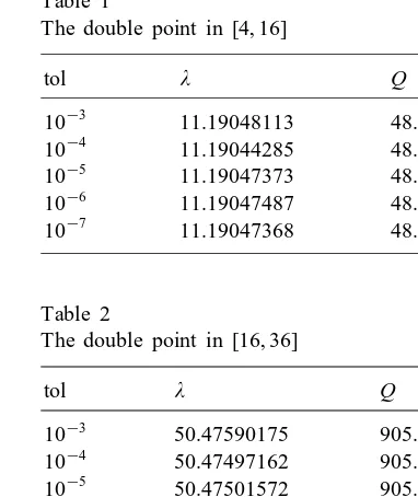
Table 1
The double point in [4;16]
tol Q
10−3 11.19048113 48.01041400
10−4
11.19044285 48.01041405 10−5 11.19047373 48.01041405
10−6 11.19047487 48.01041405
10−7
11.19047368 48.01041405
Table 2
The double point in [16;36]
tol Q
10−3 50.47590175 905.81573398
10−4
50.47497162 905.81573523 10−5 50.47501572 905.81573524
10−6 50.47501757 905.81573524
10−7
50.47501784 905.81573524
We perform our algorithm on an IBM Workstation TTX. The results are listed in Table 1. To test our results, we truncate the innite matrix A of order 100 with Q= 48:01041405. Using Matlab we have that its rst two eigenvalues are
1=2= 11:1904735991294;
These two eigenvalues merge and are very near to the double point we compute, which shows our results are credible.
We can also use the idea of our algorithm to compute the subsequent double points, though it is lacking theoretical analysis. Modifying the choice of a1 and a2 in Algorithm 1 as a1 = 0 and
a2 = 2000, we have the numerical results in Table 2.
Also if we truncate Aof order 100 withQ=905:81573524;we nd the third and fourth eigenvalve merge:
3=4= 50:47198768:
References
[1] M. Abromovich, I.A. Stegun, Hand of Mathematical Functions, Dover Pub., New York, 1965 (corrected printing, 1972).
[2] G. Blanch, D.S. Clemm, The double points of Mathieu’s dierential equation, Math. Comput. 23 (1969) 97–108. [3] I.S. Gradshteyn, I.M. Ryzhik, Table of Integrals, Series and Products, Academic Press, New York, 1980.
[4] C. Hunter, B. Guerrieri, The eigenvalues of Mathieu’s equation and their branch points, Studies Appl. Math. 64 (1981) 113–141.
[5] R.A. Lippert, A. Edelman, The computation and sensitivity of double eigenvalues, http==www-math.mit.edu=∼edelman, 1998.