GAP-CLOSING 3D BUILDING RECONSTRUCTION BY ALIGNING BOUNDARIES OF
ROOF SEGMENTS AND DETECTING UNCOVERED DETAILS
M. Pohl, D. Bulatov
Fraunhofer Institute of Optronics, System Technologies and Image Exploitation, Gutleuthausstr. 1, 76275 Ettlingen, Germany - (melanie.pohl, dimitri.bulatov)@iosb.fraunhofer.de
KEY WORDS:3D building reconstruction, polygon alignment, cut lines, step lines, boundary of roof faces, uncovered details
ABSTRACT:
We describe a work flow to border building faces which aims to obtain a detailed and closed building model. Initially, we use the estimated roof planes and the rasterized binary mask of the corresponding inlier set to generate bordering polygons. To close the gaps between the initial boundary polygons and between the polygons and the building ground outline, we introduce an algorithm to align boundaries which successfully works in 2.5D and 3D. To enhance the accuracy of the boundary alignment, we use additional reliable model entities such as cut lines and step lines between the initial estimated roof planes. All gaps that cannot be avoided by this procedure are afterwards covered by a method searching for uncovered details.
1. INTRODUCTION 1.1 Motivation and Preliminaries
Modeling single buildings as well as cityscapes is a wide topic considered in research for civil security, disaster management or just to ensure a recognizable scene representation. For some to-pics like geometrical analysis as computation of volumes, it is necessary to guarantee an instance of a building model to be closed and its building faces must not contain holes or gaps as well. Hence, we are interested in obtaining as complete as possi-ble model instances of buildings.
We assume the availability of segmentation results of the given point clouds into topographic object types such as buildings, veg-etation and ground. Procedures for building detection are given in (Bulatov et al., 2014, Lafarge and Mallet, 2012). Furthermore, we assume that the building faces consist of planes and the plane parameters are given. In our case, the dominant planes are usually computed by means of the multi-model RANSAC (Fischler and Bolles, 1981) or J-Linkage (Toldo and Fusiello, 2008), because these methods are robust against noise in the data. However, due to the inlier thresholds, several smaller plane segments may get lost during the plane estimation process.
Our task is to fill the gaps between neighboring plane segments and between plane segments and the corresponding building out-line. We will use cut lines and step lines resulting from the ini-tially estimated planes as reliable model entities. The challenge is to close the gaps between the plane segments and to preserve these geometric entities and therewith a high level of detail of the building parts.
Of course there are several state-of-the-art approaches about gen-erating low-poly 3D model instances as we will describe in the following section. These related works are able to deal with the complex structure of modern European architecture, but it often have deficits by treating flat roofs especially if there are build-ing parts with smaller flat roofs, includbuild-ing again smaller elevated (flat) structures. We will introduce an algorithm that works on these building parts well without oversmoothing.
1.2 Contribution and Related Works
Our approach is a bottom-up, or data-driven approach.
Starting from point clouds and plane parameters, rules are used to obtain a regularized output. However, we refer to a model-driven approach (Elberink and Vosselman, 2009): First, it is interest-ing because of the case study for uncovered details in Sec. 6. and second, we used large parts of the graph structure needed to deter-mine neighborhoods of boundary polygons. One significant dif-ference between our work and the building polygonization step of (Sohn et al., 2012, Bulatov et al., 2014, Lafarge and Mallet, 2012) consists in the ability of our algorithm to handle both 2.5D point clouds, represented by the altitudez = f(x,y)as a func-tion of longitudexand latitudey, and scattered point clouds in 3D space. In (Lafarge and Mallet, 2012), the outlier percentages are extremely low. This is why the authors rely on the initial polygonization of the inlier sets and do not consider neighboring relations of the polygons. The method of (Gross et al., 2005), to model roof polygons, is the core procedure of (Bulatov et al., 2014) and considers pairwise intersections of planar segments.
Three main problems may occur: First, buildings with several flat roofs of different heights are wrongly reconstructed as shed roofs. Secondly, smaller roof parts like dormers are oversmoothed by the surrounding roof parts. If there are smaller lowered roof struc-tures or shafts, these parts are closed by a continuous plane seg-ment of the surrounding higher roof parts. Third, the polygoniza-tion is done by a continuapolygoniza-tion of dominant line segments starting from the longest detected line continuing over neighboring lines and closing the polygon. Doing so, this could lead to polygons that may extend over several roof segments and missing cut lines lead to degenerated polygons that exclude large parts of a roof segment.
We will extend the algorithms to handle these special cases that play an important role in the process of building reconstruction. This delivers a more exact result with more detailed and locally more precise plane and polygon segments and therefore a much better and more realistic visualization.
The work of (Reisner-Kollmann et al., 2011) considers the case of 3D polygons embedded into 2D space and use line segments detected in images for aligning the polygons, but not many details are given about filling uncovered regions dealing with spurious lines – for instance, lines in 2D but not in 3D – which do not contribute to the improved geometry.
2. INITIAL POLYGONIZATION
A polygonP ∈R2×nconsists of an ordered set ofnverticesV=
{v1,v2, ...,vn}and edgesE={e1,e2, ...,en}. So, a polygonPis a sequence of vertices and edges so that every vertex is of valence two and all upcoming calculations on polygonal subscripts are to be interpreted modulon.
Most state-of-the-art 2.5D approaches use the binary mask, called bitplane, from all(x,y)values that belong to the inlier set, usu-ally post-processed by morphological operations. For the binary mask a contour-following algorithm is applied. The contour of the generated bitplane is used as theinitial polygon. However, even in the 2.5D case, the binary masks of slanted polygons are strongly distorted and do not reflect reliable information on their extensions. Since in 3D this problem becomes even more dra-matic, we decided to prepare the binary mask for each individual polygon in its own coordinate system specified byuandv. We achieve an orthogonal projection of all points labeled as inliers of a dominant planefby two rotations around thexandyaxis. The product of two rotation matrices is denoted byR. Afterwards, we translate the polygon in theuv-plane such that the convex hull of the transformed point cloud lies completely in the first quad-rant. The corresponding 3×3 matrix is denoted byT. Finally, a uniform scalingSis applied to represent the binary image at a resolution which depends on the sampling densitiy. All points of the set of inliersXare projected by
P=S T[R03], 2Dx=P3Dx, 3Dx∈ X (1)
into the local coordinate system while03is the 3×1 zero vector.
The values of the binary mask at their rounded pixel positions are set to 1, otherwise, they are 0. In order to transform points from theuvintoxyzcoordinate system, we apply the transformation
Q=P∗−c(fP∗)/(f c), 3D x=Q2D
x (2)
whereP∗ is the pseudo-inverse of the 3×4 matrixPfrom (1) andcis the one-dimensional kernel vector ofP. All variables are in homogeneous coordinates. The way from the binary masks to initial polygons is the same as proposed by (Reisner-Kollmann et al., 2011, Gross et al., 2005). All calculations take place on polygons in 2D while constraints are obtained in 3D.
Because every polygon corresponds to the boundary of one pla-nar roof segment and due to noise in the data, neighboring poly-gons often do not share edges intended. Occurring gaps between neighboring boundary polygons will be removed by shifting ver-tices within our aligning procedure described in Secs. 4.-7. Be-fore going into detail, it is necessary to introduce the concept of neighborhood, as will be done in the next section.
3. NEIGHBORHOODS
3.1 Obtaining cut lines and step lines from the graph The building faces represented by polygons can be interpreted as a graph. A graph is a representation of a set of objects, called graph-vertices, where some pairs of objects are connected by
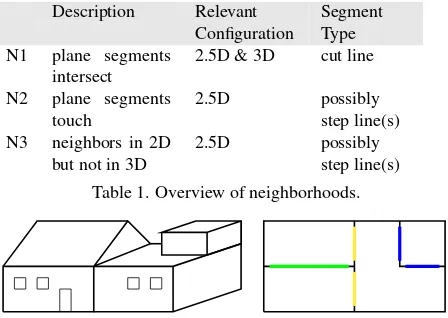
Description Relevant Segment
Configuration Type N1 plane segments
intersect
2.5D & 3D cut line
N2 plane segments
Table 1. Overview of neighborhoods.
Figure 1. Neighborhood of roof segments: The left figure shows the 3D building, the right figure shows the building from the bird’s eye view. Green: Two segments intersect in a cut line (N1); yellow: two segments touch each other in a point or a segment of insufficient length (N2); blue: two segments are neighbors in 2D but not in 3D (N3).
edges. In our case, the graph-vertices are dominant planes that are limited as described in Sec. 2. To anticipate, this limitation results in a boundary polygon. The graph edges are different kinds of neighborhoods among the roof segments. The structure of the graph is thus similar to that of (Elberink and Vosselman, 2009) though we have less neighborhood types. The approach to achieve a pre-selection of candidates for adjacencies in the graph is different for 2.5D and 3D configurations: For a 2.5D configura-tion, we use the bitplane in 2D (that is 1 for each pixel inside the footprint of the boundary polygon) and expand each segment by a morphological dilatation. The overlap of two bitplanes is used to extract the neighbors in 2D. For a 3D configuration, the pre-selection of planes can be achieved by comparison of 3D bound-ing boxes for each initial 3D polygon. If two boundbound-ing boxes in-tersect, the ultimate check is performed using the Approximated Nearest Neighbors algorithm (Arya et al., 1998).
Consider a pair of planesf1 andf2 spanning a 2D vector
sub-space. We denote the pair of vectors spanning the orthogonal complement of this subspace byv1andv2. Then the intersection
line off1,f2projected by the cameraPinto an image is given by
l= (Pv1)×(Pv2). (3)
This is valid both for 2.5D and 3D configurations and can handle also intersection lines at infinity resulting from parallel planes. For a 2.5D configuration, the matrixPis given by
P=
and in the case of a 3D configuration,Pis the synthetic transfor-mation of either plane.
these neighborhood types by N1 (segments intersect in a line seg-ment, called cut line) and N2 (touching segments), respectively.
If, in contrast,llies far away from the vertices of one of the two boundary polygons, the corresponding plane segments neither in-tersect nor touch. This case could e.g. occur iff1 and f2 are
parallel flat roof segments of different heights. Hence, they are neighbors in 2D but not in 3D caused by the difference in height. This type of neighborhood is denoted by N3.
For the neighborhood types N2 and N3, which are only valid in 2.5D configurations, we consider, additionally to cut lines, straight line segments at elevation jumps, called step lines. To do so, straight line segments in a smoothed DSM are computed by the method of (Burns et al., 1986). Considering a narrow rect-angle around the line segmentls, we check if it lies inside a build-ing. If so, we assert iflslies near one or more pairs of polygons and select only those pairs for which the majority of points in the polygons lies on different sides ofls. Finally, the line segment is clipped in order to fit the boundary polygon extension.
We summarize the neighborhood relations of polygons together with the resulting line segments in Tab. 1 and Fig. 1. The line segments resulting from the neighborhood of type N1, N2 and N3 are visualized by green, yellow, and blue lines, respectively.
We consider the line segments to be “true” representatives for the roof segment borders. To close the gaps between neighboring boundary polygons of particular kind or to remove the overlaps, the boundary polygons will be aligned to these line segments in the proposed procedures. Because the alignment of the boundary is for that case just a 2D problem, we can ignore the height infor-mation and further treat cut lines and step lines in the same way. To close the gaps to the building outline, it will be necessary to align each polygon also to the building outline.
3.2 Merging step lines
The last pre-processing step – merging step lines – is needed to avoid splinted segments which can cause holes during the align-ment. Furthermore, step lines being incident to e.g. N1-neighbor-ing polygons (see yellow step lines in Fig 1) are supposed to be collinear and therewith can be replaced by one longer single line segment. We will merge these step lines to a longer line segment and use this line segment for all incident building faces. For this reason, we do not just merge the step lines being incident to one polygon but all step lines that are incident to each pair of neigh-boring polygons. Since the neighborhood graph already depicts possible corresponding line segments, we use the following work flow:
1. For one pair of neighboring polygons (N1, N2 and N3) col-lect all segments of incident step lines.
2. Search for segments of step lines that are collinear within a certain threshold (typically 5-10◦).
3. Choose one segment of step line from this set to represent the reference vector−AB−→and one of its endpoints (without loss of generality, we chooseA) as reference point.
4. For each other segment from step 2 and each endpointS1
andS2of these segments, determine
−−−→
AS1and
−−−→
AS2and
de-fine them as bonding vectors.
5. If the angles between this bonding vectors and the reference vector do not exceed the given threshold, merge the seg-ments by replacing the considered pair of segseg-ments by the segment given by the pair of points with the largest distance.
(a) DSM of a synthetic test building
200 250 300 350 400 450 500 150
200
250
300
350
400
450
500
(b) cut lines and unmerged step lines
200 250 300 350 400 450 500 150
200
250
300
350
400
450
500
(c) cut lines and merged step lines
Figure 2. Merging step lines: If a step line is splinted (e.g. upper right, light green and blue), they get merged. Cut lines (dotted) are not merged.
Ptarget Ptrigger
? <bϑ
6. Continue with 3. until all segments are tested.
7. Continue with 1. and the next pair of neighboring polygons.
An example for merging step lines generated from the DSM in Fig. 2(a) is shown in Fig. 2(b), 2(c). The splinted step lines in the upper right (blue and light green), in the upper left (blue and red), in the lower left (black and green) and in the lower right part (purple, blue and red) are replaced by single representatives, respectively.
In principle, we could apply this algorithm to cut lines as well but modern architecture often offers parallel pairs of N1-neighboring roof segments with slight offset. Hence, we use the merging al-gorithm only for the step lines.
With these prearrangements, we now introduce the work flow for the alignment process.
4. ALIGNMENT
This section handles adjusting polygons representing building fa-ces, which we callPtrigger, to fixed polygons, that is, building outlines, cut lines and step lines that are calledPtarget. Note that a 1D line segment is merely a degenerated polygon, but because of a mostly analogous approach, we will also refer to lines as polygons as well. In the following, we will always look to the suitable – in the sense of Sec. 2. – 2D projection of a polygon.
4.1 Changing Vertex Positions
As introduced, Ptarget is the fixed polygon, while the polygon Ptriggerwill be aligned toPtarget. At first, we define a threshold
ϑof distance. If the Euclidean distance between a vertexvjof
Ptrigger and an edge ofPtarget is less thanϑ, and the projected vertex is an inner point of that edge, the residual of the projection of this vertex onto the edge ofPtarget is computed. In a second step, for each projection the one of the smallest residual is kept. So, for every vertexvjthe aligning process is a functiona:R27→
R2with
The variablesvekj are the orthogonal projections ofvjto thek-th
edge ofPtargetandv0jis the non-projected initial vertexvj.
In a vectore, we store the information which vertex ofPtriggeris projected to which edge ofPtarget(e(j) =k, ifvjis projected to edgek;e(j) =0, if the vertexvjis not projected).
We introduce a special projection rule in the case thatPtarget is a line: In general, a vertex that has an appropriate distance to an edge is only projected if its projection ispart of that edge, so is an inner point of it. In the case thatPtargetis a line segment, we allow a tolerance zone of radiusrϑaround each incident vertex, so that the projected vertex ofPtriggeris allowed to lie “outside” the edge.
This process of alignment leads to some special configurations that need to get a further treatment that is introduced in the fol-lowing subsections.
4.2 Delete Vertices
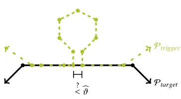
In a next step, we consider the non-projected vertices ofPtrigger. Sometimes,Ptriggermay form a bubble (see Fig. 3). A bubble is formed if two vertices ofPtriggerare projected to the same edge ofPtarget within an intra-edge distance below a given threshold
b
ϑand there is just a maximal number of non-projected vertices in between. These vertices are deleted fromPtrigger.
Letnbe the maximal number of vertices that are allowed to be deleted. There existi, jwithi< jand 1 < j−i≤n+1 with
kPtrigger(i)− Ptrigger(j)k<bϑ∧e(i) =e(j). Then used:R27→
R2with
d(Ptrigger,i,j):Ptrigger= [v1∗, ...,v∗i,v∗j,v∗g] (6)
g=|V∗|.
The previous introduced *-marker consequently is eitherekor 0, depending on the projection.
4.3 Insert Vertices
In case,Ptargetis the building outline it is also possible to insert vertices toPtrigger in order to add corners, namely the incident vertex of the edgePtarget.
Vertices are inserted if the following conditions hold
e(i) = j ∧ e(i+1) = j±1
5. DEALING WITH SELF INTERSECTIONS, OVERLAPS AND FOLDINGS
Unfortunately, the introduced procedures (a, d, w) may change the morphologic sequence of the vertices inPtrigger and lead to polygon self intersections, overlaps and foldings that we summa-rize under the termtwist. Therefore, we introduce a “cleaning”-method for the resulting polygons. As a twist, we understand one of the following situations (see Fig. 4):
(a) Eis the set of edges inPtrigger. If there exist two edges
eiandej ∈ Ethat intersect in one point which is not their common incident vertex, the polygon forms areal twist.
(b) Lete0 be the non-zero entries of e. If there existk,l ∈
1, ...,|e0|, k<land eithere0(l)<e0(k)in case of a positive
direction of passage ofeaccording toPtarget(meaning, the non-zero labels ineare increasing) ore0(l)>e0(k)in case
of a negative direction of passage,Ptriggerforms abackward
projectionto a previous edge.
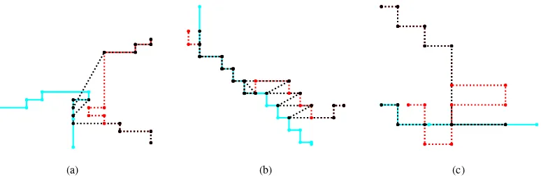
(a) (b) (c)
Figure 4. Types of twists: a) real twist; b) backward projection; c) leak. The light blue polygon denotesPtarget, the red polygon the initialPtriggerand the black polygon denotes the projectedPtrigger.
v1 v2
v3
v4
ei
ej
Figure 5. Ambiguous possibilities to remove the twist in the aligned polygon. By just deleting one of the vertices that are in-cident to the twisting edges, the area of the polygon will change differently. Red: numbered initialPtrigger, light blue: part of Ptarget, black: resultingPtrigger.
The following sections depict a way to eliminate these twists in the output of the alignment.
5.1 Real Twists
Since twists occur only as a consequence of projections within a certain threshold, there cannot occur arbitrary twists in the whole polygon. In this task, just two groups of this type of twists arose:
1. ∃vek i , v
ek
j, i < jand∃m, i< m < jwithe(m) = r ,
k, e(m),0⇒ver
mdefines a misprojection.
2. ∃veki , veki+1and the incoming edge ofveki intersects the out-going edge ofvek
i+1⇒v
ek i , v
ek
i+1form a twist caused by
pro-jection in the wrong order.
The first type is eliminated at the beginning of the algorithm, the second at the end. This is done because the second type can also be produced by eliminating backward projections and leaks.
Real twists type (1).Caused by the alignment of one polygon to the other one, the assigned non-zero edge labels of a well-formed polygon should either be increasing or decreasing and all vertices of the same edge label must not be separated by other labels than zero. For detection of real twists of type one, we collect all ver-tices between the first and the last projected vertex of the same label. If there exist vertices in between with other (non-zero-) la-bels, the incident edges of these and the surrounding vertices are supposed to form a twist. Cleaning these twists is ambiguous (see Fig. 5), because there are many possibilities to remove the twists from the polygons. In this example, the result of edge labels after
ei
e= (0,ei,ei, 0)
ei
1 2
3 4
1 3
2 4
(a) Real twists type 2: Re-moving twists by renumber-ing.
a vi+4vi+3 vi vi+1vi+2 vi−1
(b) Leak: Keeping vertices vi and
vi+4 as the locally first and last pro-jected vertices eliminates the leak.
Figure 6. Removing real twists of type 2 and leaks.
the alignment ise= (ei,ej,ei,ej). So, there existvei1,vei3 butv ej
2,
as well asvej2,vej4 butvei
3 that form a real twist of type 1. With high
probability, vertexv1has to be projected to edgeeiand vertexv4
to edgeejbecausea(v1)anda(v4)have by far the smallest
resid-uals. Deletingvej
2 by applyingd(Ptrigger, 1, 3), as a consequence
of the “wrong” edge label in the group of vertices that are pro-jected to edgeeiis a solution to the problem, but leads to a large change in area of the polygon. We lose the purple area and add the green one. The vector of edge labels results ine= (ei,ei,ej). A little lower change in area occurs, when deleting vertexvei
3 with d(Ptrigger, 2, 4),e= (ei,ej,ej), instead. Although this does not fit to the introduced rule, it would be a consequence of the high-est uncertainty in projection of vertexv3that has almost the same
distance to edgeeiand to edgeej.
It is hard to figure out a global rule to remove vertices concerning distances of original input vertices and projected vertices, or ver-tices among each other as well as changes in areas. We decided to remove the twist by introducing a further thresholdκand first pro-jecting the vertex in question (here vertexv2) to the “right” edge.
If the distance between the original input vertex and its projection exceedsκ, the vertex will not be projected and the input vertex is used instead, otherwise we replace the “wrong” projected vertex by the projection to the “right” edge.
Figure 7. Simulation of an uncovered detail – left: the blue ob-ject is reconstructed, but the upper front part is missing. Adding an area of the uncovered detail leads to two possibilities. Either a segment is adjoined and specified by the surrounding recon-structed edges (middle), or the area is continued by expanding one of the surrounding plane segments (right).
5.2 Backward Projections
Backward projections are easy to detect ine, too. Inethe non-zero entries are only allowed to increase or to decrease. All ver-tices that do not have appropriate edge labels will be deleted.
5.3 Leaks
The elimination of leaks can be done without their explicit detec-tion. Because of the linearity of an edge and thereby the linear dependency of all successive vertices that are projected to that edge, it is sufficient to keep the first and the last projected ver-tex of each projected group. All interior vertices are then deleted from the vertex-set. With this procedure, we eliminate leaks in the polygons as shown in Fig. 6(b). This is possible due to the fact that a leak has always a forerunner and a follower being pro-jected to the same edge.
In the whole procedure, it has to be taken in account that there can be a jump in the edge labels from the maximal edge label to the minimum edge label or vice versa.
6. UNCOVERED DETAILS
For 2.5D configurations, the ground polygon of the building is usually available. By computing the difference between the in-terior of the ground polygon and the union of the polygons ob-tained so far, we extract the details to which no plane has been assigned. We refer to those which have a non-negligible area and not too high value of eccentricity asuncovered details and we wish to find a corresponding plane for each uncovered detailU. First, we determine adjacent plane segments toUin 2D and com-pute the percentage of points ofUapproximately incident with the plane corresponding to these segments. We assign toUthe plane with the maximal percentage of inliers, if its value exceeds 60%. Otherwise, we compute a single dominant plane approxi-mating points insideUand if its inlier percentage exceeds 60%, we compute the 3D coordinates of the vertices ofUby means of this plane, otherwise it is ignored and set as an exterior part of the building. A schematic diagram is given in Fig. 7.
7. GENERALIZATION
Dealing with uncovered details often leads to a creation of a high number of additional edges. Furthermore, the bordering polygons have a high number of edges in non-aligned parts of the polygon. To reduce their number for modeling, a step of generalization follows. We apply the algorithm of (Douglas and Peucker, 1973) but allow only the generalization of successive verticesv0j. If the generalization would be applied on all points, this step could destroy the alignment.
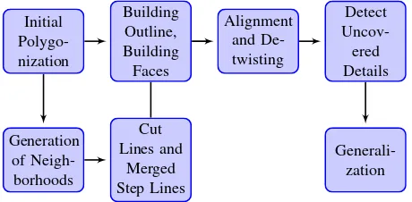
To summarize the alignment process, an overview of the specified thresholds is given in Tab. 2 and the work flow is given in Fig. 8.
ϑ euclidean distance to align
one point to an edge
dependent of the poly-gons second largest ex-pansion (∼20%) rϑ ”outside”-edge tolerance if
Ptargetis a line
1
b
ϑ threshold to delete bubbles 1.5ϑ
n number of vertices allowed to be deleted
4-8
κ distance for elimination of
twists
1.5ϑ
Table 2. Table of given alignment thresholds with short descrip-tion and empirically determined decision rule. The values are given in pixels by building polygons of a resolution of around 15cm per pixel.
Figure 8. Workflow of the proposed method from the initial poly-gon to the generalized output. The building outline as well as cut lines and step lines serve as target polygons, the initial polygo-nization of the building faces serve as trigger polygons.
8. RESULTS
We generate a synthetic building to compare our aligning algo-rithm with the initially mentioned algoalgo-rithms. This synthetic ex-ample combines a lot of real roof structure challenges other build-ing reconstruction methods yield non-optimal results so far.
The digital surface model (DSM) of the building is shown in Fig. 2(a). There are four flat roofs on the edges that pairwise en-close four saddle roofs paired with some noise. Three of the four flat roofs feature smaller flat roof structures: Two upper ones (top left and right) and one lower one (bottom right). The bottom right flat roof also contains an area of stronger noise (bottom left cor-ner). The average height of the larger flat roof areas is 10m, the saddle roofs are up to 2m higher.
As thresholds for the alignment, we useϑ = 4, rϑ = 1, bϑ = 2ϑ, n=5.
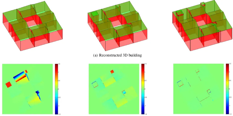
The results of the different reconstruction methods are shown in Fig. 9. Fig. 9(a) depicts the reconstructed 3D view of the building using the detected plane segments (confined by the aligned poly-gons). The walls are constructed by drawing orthogonal plane segments to the ground from the borders of each polygon.
(a) Reconstructed 3D building
(b) Quality control of the reconstructed plane segments in comparison with the ground truth.
Figure 9. Results of the building reconstruction concerning the DSM in Fig. 2(a). Left column: Results with line continuation, cut lines and multiple building agglomeration; middle column: Results by using additional step lines; right column: Polygon based results using cut lines and step lines and a single building approach.
on the flat roof in the upper and lower right. The corresponding planes from remaining data points lead to shed roofs.
In Fig. 9(b) the differences of the ground truth building faces and the estimated plane segments are shown.
The maximal deviation in the upper saddle roof and in the low-ered right flat roof is±1, 5m. This is the value, the reconstructed plane segment diverges (higher or lower) from the ground truth segment. Even, if there are many parts that diverges lesser, there are big areas where the reconstructed plane segments do not fit to the ground truth.
The second approach (Fig. 9, middle) considers step lines, too. By adding this type of lines, the elevated and especially the low-ered building parts can be reconstructed. The remaining question is how to get these step lines. If some of them are not detected, the resulting building will be malformed.
Finally, our approach shows the most exact results by consider-ing the alignment of borderconsider-ing polygons. All parts of the roofs – and especially the flat roofs with the smaller elevated and low-ered parts – are detected correctly and the estimated planes fit well. The only mismatch can be detected at some border areas in form of very thin (one pixel wide) tubes. This may be caused by a slight mismatch of some step lines by one pixel. The most im-portant task of a correctly reconstructed topology of the building is fulfilled. Even the part of stronger noise is obtained correctly with an uncovered detail.
We are testing our method also on a real data set of Meppen, Germany. This data set consists of 114 buildings and is well-suited for our purpose because it includes many buildings with flat roof structures. From this data set, a digital surface model and a classification into buildings, vegetation and ground is extracted.
Starting with the initially estimated planes, we calculate the cut lines and step lines and useϑ=4,bϑ=1.5ϑ, n=5, rϑ=ϑas alignment thresholds.
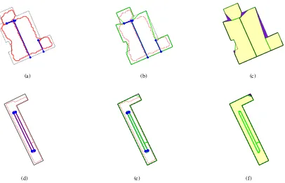
The method worked well for most buildings and is demonstrated here on two examples: In Fig. 10(a), the extracted ground poly-gon (black) as well as the initial estimated boundary polypoly-gon (red) of the roof segments are shown. After aligning each initial polygon to the cut lines and step lines as well as to the building outlines, we obtain the green polygons shown in Fig. 10(b). The corresponding covered areas are depicted in Fig. 10(c) by yellow areas. First, the purple areas are missing, but it is possible to cover them afterwards by using the technique for uncovered ar-eas (see Sec.6.). The lower left uncovered area could be avoided by using a slight higher threshold to insert vertices. Since we do not only care on single buildings but on whole data sets, these situations can always occur and be covered afterwards. Another building of the Meppen data set is shown in Fig. 10(d)-10(f). The inner elevated flat roof can be outlined from the surrounding flat roof. We detected two step lines shown in blue. Since the smaller step lines are missing, the polygon alignment seems to bee little frayed. Nevertheless, all roof polygons can be detected correctly and the whole building polygon is covered in the end.
Considering the impact of noise, we go back to the initialization of the polygons: The polygons are generated based on the esti-mated planes. Moderate noise level can be ignored or compen-sated by the plane estimation algorithm. At a high level of noise, additional planes may be estimated in noisy areas which lead to the initialization of small boundary polygons. Since normally these polygons are too small, they will be deleted and modeled as uncovered details after the alignment. For example, the noisy area in the lower left corner of the lower right flat roof of Fig. 9 (right column) is omitted and is later merged with a boundary polygon as an uncovered detail.
9. SUMMARY AND OUTLOOK
(a) (b) (c)
(d) (e) (f)
Figure 10. 2D representation of building outline and bordering roof polygons of two buildings of the data set Meppen. Left column: generated building outlines (black), initial bordering plane polygons (red) and corresponding cut lines and step lines (blue); middle column: aligned bordering plane polygons (green); right column: The covered area is depicted in yellow. The purple areas are missing firstly but can be added by processing uncovered details.
boundary polygon that should definitely be included. All other parts of the polygons are aligned to that lines or to the ground polygon. If there are still some areas missing, we can close the gaps by searching for uncovered details.
In the future, it will be necessary to further refine this procedure. Some areas that cover parts outside the building ground polygon (see Fig. 10(c), left) should be eliminated. Although the initially constructed polygon is malformed and leaks the ground polygon of the building, a not detected cut line or step line may cause multiple covered regions. Furthermore, we want to extend the number of reliable model entities by intersection points of three or more initial estimated neighboring planes. These intersection points shall be included additionally to cut lines and step lines to enhance the accuracy of the limiting border of the building faces.
To avoid twists from the beginning, it is conceivable to include a smoothness term into the alignment procedure. Each vertex ofPtriggger does not have to be aligned to the nearest edge of Ptargetbut to the most plausible one, taking the alignment of the surrounding vertices in account.
REFERENCES
Arya, S., Mount, D. M., Netanyahu, N. S., Silverman, R. and Wu, A. Y., 1998. An optimal algorithm for approximate near-est neighbor searching fixed dimensions. Journal of the ACM (JACM) 45(6), pp. 891–923.
Bulatov, D., H¨aufel, G., Meidow, J., Pohl, M., Solbrig, P. and Wernerus, P., 2014. Context-based automatic reconstruction and texturing of 3d urban terrain for quick-response tasks. ISPRS Journal of Photogrammetry and Remote Sensing.
Burns, J., Hanson, A. and Riseman, E., 1986. Extracting straight lines. IEEE Transactions on Pattern Analysis and Machine Intel-ligence 8(4), pp. 425–455.
Douglas, D. H. and Peucker, T. K., 1973. Algorithms for the reduction of the number of points required to represent a digitized line or its caricature. Cartographica: The International Journal for Geographic Information and Geovisualization 10(2), pp. 112– 122.
Elberink, S. O. and Vosselman, G., 2009. Building reconstruction by target based graph matching on incomplete laser data: analysis and limitations. Sensors 9(8), pp. 6101–6118.
Fischler, M. and Bolles, R., 1981. Random sample consensus: A paradigm for model fitting with applications to image analysis and automated cartography. Commun. ACM, 45, pp. 381–395.
Gross, H., Th¨onnessen, U. and v. Hansen, W., 2005. 3D-Modeling of urban structures. International Archives of Pho-togrammetry and Remote Sensing 36 (Part 3W24), pp. 137–142.
Lafarge, F. and Mallet, C., 2012. Creating large-scale city models from 3D-point clouds: a robust approach with hybrid representa-tion. International Journal of Computer Vision 99(1), pp. 69–85.
Reisner-Kollmann, I., Luksch, C. and Schw¨arzler, M., 2011. Re-constructing buildings as textured low poly meshes from point clouds and images. In: Eurographics, pp. 17–20.
Sohn, G., Jwa, Y., Kim, H. B. and Jung, J., 2012. An implicit regularization for 3D building rooftop modeling using airborne LIDAR data. ISPRS Annals of the Photogrammetry, Remote Sensing and Spatial Information Sciences 2 (3), pp. 305–310.