QUASI-FIVE-POINT ALGORITHM WITH NON-LINEAR MINIMIZATION
Kazuo Oda a
a Asia Air Survey Co., Ltd.
1-2-1 Manpuku-ji, Asao-Ku, Kawasaki-Shi, KANAGAWA, 215-0004 JAPAN - [email protected]
Commission V
KEY WORDS: Five Point Algorithm, Relative Orientation, UAV
ABSTRACT:
Five-point algorithm is a powerful tool for relative orientation, because it requires no initial assumption of camera position. This algorithm determines an essential matrix from five point correspondences between two calibrated cameras, but results multiple solutions and some selecting process is required. This paper proposes Quasi-Five-Point Algorithm which is non-linear solver with seed solution of 8 point algorithm. The method tries to calculate the appropriate essential matrix without selecting process among multiple solutions. It is one of non-linear approach, but tries to find an appropriate seed before non-linear calculation. Using correspondences of 3 or more additional points, seed values of the solution is calculated. In this paper relationship between traditional parametric relative orientation and essential matrix is discussed, and after that quasi-five-point algorithm is introduced.
1. INTRODUCTION
Relative orientation is the important tool in photogrammetry. Traditional relative orientation calculates five relative orientation parameters with coplanarity constraint equations in non-linear optimization process, but without good initial values of parameters calculation goes local minimum and fails. Recently images captured from UAV are often used in photogrammetry. Unstable attitudes of UAV often cause failure of calculation of relative orientation.
Five-point algorithm, originally developed and used in computer vision field for relative orientation, is now adopted in photogrammetry filed. This method computes an essential matrix. Essential matrix is a 3 x 3 matrix which gives coplanarity constraint in following form:
(1)
where and are camera coordinates of corresponding points in a pair of images. It determines essential matrix from five point correspondences between two calibrated cameras, with coplanarity constraint and other constraints.
One type of five point algorithm (Nistér, 2004, Li et al., 2006) directly solves scalar multipliers with cubic rank constraint and the cubic trace-constraint. These methods solve tenth order of polynomial equations and provide multiple solutions.
Another type of five point algorithm is a non-linear solver (Batra et al., 2007), where translation vector and the four scalar multipliers are solved with non-linear minimization.
This type of method can obtain more accurate result than algebraic approaches, but requires multiple seeds to get multiple
solutions. Thus five-point algorithm requires users to choose the right solution among the multiple solutions, with checking cheirality or re-projection errors of other point correspondences (Dodehorst et al., 2008).
This paper proposes Quasi-Five Point Algorithm which is non-linear solver with seed solution of 8 point algorithm. This method tries to calculate the appropriate essential matrix without selecting process among multiple solutions.
Our method is one of non-linear approach which tries to find an appropriate seed values before non-linear calculation. Using correspondences of three or more additional points, our method calculates seed values of four scalar multipliers.
In this paper, relationship between traditional parametric relative orientation and essential matrix is discussed. After that new normalization method of essential matrix is proposed. Utilizing this normalization, quasi-five-point algorithm is introduced and some numerical tests show that this method can obtain more precise result than algebraic type method.
2. COPLANARITY CONSTRAINT, RELATIVE ORIENTATION AND ESSENTIAL MATRIX 2.1 Definition
Coplanarity constraint is traditionally expressed in photogrammetry as following: Let the point and are two optical center of stereo pair camera, and one point in 3D space is projected on each sensor plane. Let 3D coordinates of two projected positions be
and , coplanarity constraint is represented in following equation:
(2)
This equation means one of 4 points can be expressed by linear combination of the other 3 points in projective space.
In computer vision field, coplanarity constraint can be represented as condition that scalar triple product of three vectors , and comes to zero. This means the volume of a parallelepiped defined by the three vectors is zero. Let mean cross product and mean dot product,
(3)
By expanding left side of equation (2) and (3), one can see these two equations are the same.
Essential matrix gives the relationship between two camera coordinates of the corresponding points on the sensor. Let the camera coordinate system of the first camera be the base 3D coordinate system, and , be the rotation matrix of second camera relative to base coordinate system, and be the focal lengths of two cameras, and
With the following representation of cross product:
(5) coplanarity constraint can be written in the following equation:
Here essential matrix is defined as 3 x 3 matrix:
(7)
Thus an essential matrix gives relationship between two camera coordinates of a pair of corresponding point on the sensors:
(8)
This equation cannot fix the scale of E, thus E is generally defined up to a scale factor.
Let rotation matrix be the following expression: (9)
Using two rotation matrix relative to the base coordinate system, an essential matrix has following expression:
The rank of essential matrix is zero:
(13)
This is obvious because:
(14)
2.2.2 Cubic Trace Constraint
Essential matrix satisfies the following cubic trace constraint: (15)
This can be proved as follows. The trace is similarity-invariant,
(16)
(17) Notice that:
= (18) This leads:
(19)
2.2.3 Arbitrariness in Rotation around Line through Two Optical Centre
Essential matrix has arbitrariness with rotation around line through two optical centres:
(20)
This means that essential matrix is defined with 5 rotation angles and we can set .
2.2.4 Multiple Configuration for an Essential Matrix An essential matrix has following features:
(21)
(22) Where
(23)
The equation (22) and (23) one and the third equation is essentially the same because essential matrix has arbitrariness with rotation around line through two optical centres and:
(24)
With combination of 1) and 2), there are four geometrical possibilities for one essential matrix (Hattori et al., 1993, Hartley et al., 2003). The valid solution is the one of them where all corresponding points exist in front of the both cameras.
3. NORMALIZATION OF ESSENTIAL MATRIX
Introduction of normalization of essential matrix is convenient for evaluating precision of calculated essential matrix. Well-used method is scaling an essential matrix with Frobenius norm, that is:
(25)
We propose Quasi-Five-Point Algorithm which is non-linear solver with seed solution of 8 point algorithm. This method tries to calculate the appropriate essential matrix without selecting process among multiple solutions.
With coplanarity constraints with five point correspondence, essential matrix can expressed in following style:
(31)
where is the basis for the right null space, and are the four (arbitrary) scalar multipliers (Nistér, 2004, Li et al., 2006). Our method calculates scalar multipliers with non-linear optimization where an appropriate seed is found before non-linear calculation. Using additional 3 or more point correspondences, our method calculates seed values of four scalar multipliers with equation (29) and equation (30). This means the method directly calculate a normalized essential matrix .
After calculation of seed values of scalar multipliers, non-linear least square optimization of scalar multipliers is executed. Ten equations, which are Equation (29) and nine equations from Levenberg-Marquardt method is adopted in this algorithm for this optimization. This is beacase, in pre-testing, Levenberg- Marquardt method worked better than Gauss-Newton minimization.
Quasi-five-point algorithm cannot get good initial values in case of perfectly planar 3d scene, because the calculation of seed values fails because of rank regression. For such cases, this algorithm provide try-and-error process with randomized seed value.
5. NUMERICAL TESTS 5.1 Case 1: Tests with Non-Planar Scene
Numerical tests had been executed with simulated data. The distance between two cameras is fixed to 1m, and 8 points are distributed in 2 m x 1 m at the distance of 1 m – 10 m from optical centres (Figure 1). Undulations of 3D point distributions had been set to 0.1 to 0.00001 relative to the distance.
Figure 1. Distribution of 3D point in the test
Optical centres
Rotation angle of two cameras had been set at random with – been executed together for the sake of comparison.
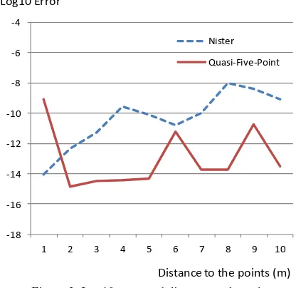
Figure 2. Log10 error and distance to the point (Non-planar scene, without noise)
Figure 2 shows relationship between distance to the point and log10 error without noise. Each error value is the mean value of 5 tests with different flatness. The figure shows that quasi-five-point algorithm is 1 or 2 order better than Nistér’s algorithm. The figure shows that errors are getting worse with longer distance from cameras to the 3D points. This is because view angle of the area where points are distributed in an image is getting smaller. Errors of quasi-five point algorithm get worse almost 2 order, but they are better than the cases of Nistér’s algorithm which get worse almost 4 order.
In this test all calculations converge on the correct values without try-and-error process. This means estimation of initial values works well.
5.2 Case 2: Perfectly Planar scene
Tests with perfectly planar scene had been also executed. Undulations of 3D point distributions had been set to zero. Rotation angle of two cameras had been set at random with – to variation in angle, – to variation in and angle, respectively. The upper limit of retry count had been set to 20 times.
Figure 3. Log10 error and distance to the point (Planar scene, without noise)
Figure 3 shows relationship between distances to the point and log10 errors without noise. The figure shows almost same trend as the Figure 2, errors of quasi-five-point algorithm at 1 m, 6 m and 9 m were worse than Nister’s. It is because they included a few cases in which non-linear optimization did not converge, or converged on incorrect values.
Table 1 shows the detail information of the test. Fifty different situations had been executed. Ninety-six % of the calculations
Table 1. Results with perfectly planar scene
Figure 4. An example of multiple solutions of five-point algorithm
The illustration shows the point distribution viewed from bottom of the y-axis, where five points lay on the same plane If two cameras are rotated around the y axis so as to two bottom edges of triangle have same z coordinate value, matching points makes parallel lines with the base line and satisfy coplanarity constraint.
6. CONCLUSION AND FUTURE WORKS
Quasi-five-point algorithm has been proposed. The tests show that the precision of the algorithm is better than Nistér’s algorithm if non-linear optimization converges on the correct value. In case of completely flat scene, nonlinear calculations obtained correct results in the rate of 92%.
The evaluation remains in noise-free case so far, so we will examine the cases with noise in near future.
REFERENCES
Batra, D., Nabbe, B. and Hebert, M., 2007. An alternative formulation for five point relative pose problem, IEEE Workshop on Motion and Video Computing WMVC '07. Li, H.D. and Hartley, R.I., 2006. Five-point motion estimation made easy, Int. Conf. on Pattern Recognition, vol. 1, pp. 630-633.
Hartley, R., Zisserman, A. 2003. Multiple View Geometry in computer vision, Cambridge University Press, second edition. Hattori, S., Seki, A, 1992. Automatic calculation of exterior orientation parameters for bundle adjustment, Journal of JSCE, No.464/IV-19, pp.139-147.
Nistér, D., 2004. An Efficient Solution to the Five-Point Relative Pose Problem, IEEE Transactions on Pattern Analysis and Machine Intelligence, 26(6):756-770.
Rodehorst, V., Heinrichs, M., and Hellwich, O., 2008. Evaluation of relative pose estimation methods for multi-camera setups. The International Archives of the Photogrammetry, Remote Sensing and Spatial Information Sciences, Vol. XYXXVII, Part B3b, Beijing .