Conference paper

Ting On Chan and Derek D. Lichti

Department of Geomatics Engineering, University of Calgary 2500 University Dr NW, Calgary, Alberta, T2N1N4 Canada

(ting.chan, ddlichti)@ucalgary.ca

LiDAR, Octagonal Pole, Geometric Modelling, Polygon

Lamp poles are one of the most abundant highway and community components in modern cities. Their supporting parts are primarily tapered octagonal cones specifically designed for wind resistance. The geometry and the positions of the lamp poles are important information for various applications. For example, they are important to monitoring deformation of aged lamp poles, maintaining an efficient highway GIS system, and also facilitating possible feature4based calibration of mobile LiDAR systems. In this paper, we present a novel geometric model for octagonal lamp poles. The model consists of seven parameters in which a rotation about the z4 axis is included, and points are constrained by the trigonometric property of 2D octagons after applying the rotations. For the geometric fitting of the lamp pole point cloud captured by a terrestrial LiDAR, accurate initial parameter values are essential. They can be estimated by first fitting the points to a circular cone model and this is followed by some basic point cloud processing techniques. The model was verified by fitting both simulated and real data. The real data includes several lamp pole point clouds captured by: (1) Faro Focus 3D and (2) Velodyne HDL432E. The fitting results using the proposed model are promising, and up to 2.9 mm improvement in fitting accuracy was realized for the real lamp pole point clouds compared to using the conventional circular cone model. The overall result suggests that the proposed model is appropriate and rigorous.

!

Roadside pole4like objects such as lamp poles are of interest for many applications such as three4dimensional (3D) city modelling and for geographic information systems (GIS). Therefore they are often the segmentation targets from large point clouds (Cabo et al., 2014; Halawany and Lichti, 2013; Pu et al., 2011; Yokoyama et al. 2011; Lehtomäki et al., 2010). However, the geometric properties of pole4like objects such as lamp poles are not modelled and estimated preciously in most cases.

If pole4like objects, particularly octagonal lamp poles, are accurately modelled geometrically, they could be treated as calibration references for terrestrial LiDAR and mobile mapping systems (Chan and Lichti, 2012, 2013; Chan et al., 2013) due to their abundance in most road scenes. In fact, developing an accurate geometric model for such pole4like objects can also be beneficial to many real4life problems such as pole reconstruction for 3D city modelling (Buhur et al., 2009), pole deformation monitoring (Chang et al., 2009) and quality control of pole manufacturing (Lindskog et al., 2012). Since most tall lamp poles usually have octagonal base and can be modelled as octagonal cones/pyramids, a rigorous geometric model of an octagonal cone is proposed in this paper.

For in situ calibration of mobile LiDAR, a rigorous 3D geometric model which equates all the x, y and z coordinates for the octagonal cone is essential and is therefore of this paper. Some research (e.g., Milenkovic, 1993) has addressed the problem of polygon modelling but the models are mostly in two4dimensional (2D) and the models and their associated constraints often consist of inequalities. Chicurel4Uziel (2004) proposed a generalized 3D model for polygonal prisms without inequality but the x and y coordinates are modelled and estimated separately using two equations and they cannot be readily expressed in terms of the other. Also, no inclinations of the prism were considered in its model.

" #

" $% & ' %( (%)

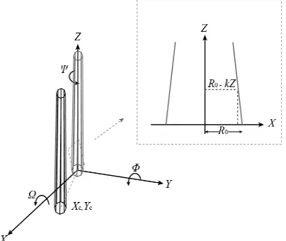
The fundamental concept of the proposed model is that by breaking the cone into many horizontal 2D octagonal layers, all eight sides of the octagon can be treated as the same one side by applying the transformation as a regular octagon is rotational symmetric. The side is then constrained with a simple trigonometric equation augmented with a half of the fixed interior angle of the octagon. The proposed model is consists of seven parameters: the cone centre (Xc, Yc), the rotations about the X4axis ( ), Y4axis (Φ) and Z4axis (Ψ), the octagonal radius (R0) at Z = 0 and also the cone gradient factor (k) as depicted in Figure 1. Some of the parameters are inherited from the conventional cylindrical model which has five degrees of freedom (Rabbani et al., 2007). The octagonal cone has one additional rotation parameter (Ψ) about the Z4axis on the top of the cylindrical model because an octagon is not isotropic about the Z4axis.

Figure 1. The parameters of the proposed octagonal cone model

45

Θ

q

=

After the cone is reduced to the origin by subtracting the cone centre (Xc, Yc), it is rotated about the X4 and Y4 axes by and Φ respectively. It is followed by further rotating the cone about the Z4axis by Ψ (422.5˚≤ Ψ≤ 22.5˚) as illustrated in Figure 2a (only showing the cross section at Z = 0) to its nominal position (Figure 2b).

Figure 2. Rotation about the Z4axis with Ψ(2a, left); The nominal position and the trigonometric constraint in the first octant (2b, right) With the octagonal cone transformed to the nominal position, points lying on the octagonal side of the first octant (red in Figure 2b) satisfy the following trigonometric constraint (1) where R0 is defined as the octagonal radius which is the distance between the centre and a vertex of the octagon on the XY4plane after the cone is transformed to be perpendicular to the XY4plane.

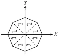
Every point lying on the cone can be classified as belonging to one of the eight octants (Figure 3) depending on the point’s position and q is defined as the octant number.

Figure 3. The octant number (q) for the model

By computing q, points lying on other octants (the 2nd, 3rd, …, 8th octant) can also be constrained by Equation (1) after rotating the points about Z4axis by the following angle

(2) nominal position by

( ) ( ) ( )

increasing height (Z). The gradient factor, k, governs the radius decrement by subtracting a small portion of Z from R0. Therefore, the overall geometric model for the octagonal cone is (5) where

(6)

Note that Equations (5) and (6) can be generalized for other polygonal cones such as hexagonal cone, which is given by

0

and n is the number of sides for the corresponding polygon.

" " * +) +&+ %*%& * +*

The initial values of all the parameters (except Ψ) of the proposed model can be estimated using least4squares fitting with the circular cone model

f

(

x

,

l

)

=

X

'2

+

Y

'2

−

(

R

₀

−

kZ

'

)

2

=

0

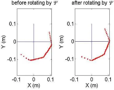
(9) except for R0, for which only a rough estimate is required (e.g. based on empirical knowledge).

After obtaining the six initial values, the cone can be reduced to the origin and rotated to be perpendicular to the XY4plane. Then the initial value of Ψ can be found by first isolating a thin octagonal layer around Z = 0 (~ 1 cm thick). This is followed by projection of the points on the layer onto a 2D image (Figure 4a). Therefore, the octagonal sides can be readily detected using region growing or the Hough Transform, and the vertices of the

(

)

( ) ( )

octagon are thus found. Ψ is the smallest angle between the X4 axis and the vertex which is the closest to the X4axis. Figure 4b shows the projected 2D image of cone in the nominal position after rotating by Ψfor 12˚.

Figure 4. Projected 2D image from the point cloud for calculating approximate value of Ψ (4a, left): before rotating by Ψ; (4b, right):

after rotating by Ψ

,

A full errorless vertical octagonal lamp pole was simulated with the realistic parameters shown in Table 1. The height of the simulated octagonal pole is 11 m and it consists of 140864 points. Figure 5 shows the simulated pole and its projected cross4section on the XY4plane Least4squares fitting of the data to the proposed model (Equation 5) was performed.

Figure 5. The simulated octagonal lamp pole (5a, left) and its projected cross section on the XY4plane (5b, right)

Table 1. The parameter values for the simulated octagonal pole Simulated Value

Xc (m) 4.2340 Yc (m) 3.5670 (rad) 40.0050

Φ (rad) 0.0060

Ψ (rad) 40.0349

k 0.0050

R0 (m) 0.1200

Five real octagonal lamp poles of two different sizes were captured with the Faro Focus 3D (Figure 6) and the Velodyne HDL432E (Figure 7) on the University of Calgary campus. The

scanner was placed approximately 4 m in average away from the poles. Least4squares fitting using the octagonal cone model (Equation 5) was performed with the lamp pole point clouds (the vertical part) captured by Faro Focus 3D (Lamp Poles 1 4 3) and the HDL432E (Lamp Poles 4 and 5). Only 4 sides of the pole were captured for each scanner position. The Velodyne point clouds contain time varying errors (Glennie and Lichti, 2011; Chan et al., 2013) and thus the least4squares convergence thresholds have to be tuned based on the severity of the noise. The details of the poles and fitting input are summarized in Table 2. The point clouds of Poles 1 and 4 are plotted in Figures 8 and 9 respectively.

Figure 6. A lamp pole was captured with the Faro Focus 3D on the University of Calgary Campus

Figure 7. A lamp pole was captured with the Velodyne HDL432E on the University

of Calgary Campus

Figure 8. The point cloud of Pole 1captured by Faro Focus 3D (8a, left) and its projected cross section on the XY4plane (8b, right)

Figure 9. The point cloud of Pole 1captured by Velodyne HDL432E (9a, left) and its projected cross section on the XY4plane (9b, right)

Table 2. Summary of the real data fitting precision from the least4squares fitting of the simulated pole. All the parameters were accurately recovered with high precision as seen in Tables 1 and 3. Also, no high parameter correlation was found from the correlation matrix (absolute value) tabulated in Table 4.

Table 3. Estimates of octagonal cone model fitting with the simulated data Table 4. Correlation matrix of octagonal cone model fitting

with the simulated data

Xc Yc Φ Ψ k R0

The mean estimated results from the least4squares fitting using the octagonal cone model for Poles 143 captured by the Faro Focus 3D are shown in Table 5. It is shown that the precisions of the parameters are all high and a reasonable estimated variance factor ( 2

0

σˆ ) is obtained (the observation standard deviations for the adjustment are listed in Table 2).

Unlike the eight4sided simulated pole, some high correlations between the parameters were found from the correlation matrix (Table 6) which shows the mean absolute values of the correlation coefficients for Poles 1 4 3. Only 4 sides (half of the pole) for each pole were observed from a scanner position and this leads to rather poor geometry for the adjustment so that R0 becomes more coupled to either Xc or Yc, or both depending the relative position between the pole and the scanner. Similarly, k is more coupled with the inclinations of the pole due to lack of observations of the complete pole. Fitting the same data to a circular cone also incurs these high correlation problems.

Table 5. Mean estimates of octagonal cone model fitting with the real data (Pole 1 4 3) captured by the Faro Focus 3D

Est. Value Std. Dev.

Table 6. Mean correlation matrix of octagonal cone model fitting with the real data (Pole 1 4 3) captured by the Faro Focus 3D

Xc Yc Φ Ψ k R0 delivered higher precision for all the parameters. Furthermore, the root mean square (RMS) values of the octagonal model fitting residuals are also lower in all the three dimensions. Up to 2.9 mm mean RMS discrepancy between two models’ residuals was realized as shown in Table 8. As a result, the proposed model is a more accurate and thus more appropriate for modelling the octagonal lamp pole point clouds.

Table 7. Comparison of the mean estimated standard deviations of the octagonal and circular cone models fitting with the real data (Poles 1 4

3) captured by the Faro Focus 3D Octagonal Cone

Table 8. Comparison of the mean RMS of the residuals of the octagonal and circular cone models fitting with the real data (Poles 1 4 3) captured

by the Faro Focus 3D Mean RMS of Residuals RMSx (mm) RMSy (mm) RMSz (mm)

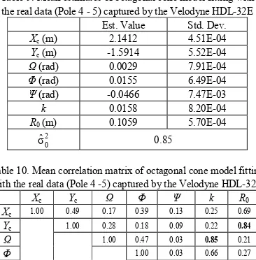
For the Velodyne point cloud for Poles 4 4 5, the fitting with the octagonal cone model also gives realistic estimates (except k) with high precision and also a small estimated variance factor as shown in Table 9. The estimated k is large because the differences between systematic errors adherent to the points captured by different laser heads are high and this causes the

whole point cloud deviated extensively from the conic structure in which the radius is reduced by a small fixed ratio (k) when the vertical position increase. Furthermore, the parameter correlations are fairly low except the 4k and Yc4R0 correlations as seen in Table 10. A similar conclusion from Section 4.2.1 can be drawn for explaining that.

Table 9. Mean estimates of octagonal cone model fitting with the real data (Pole 4 4 5) captured by the Velodyne HDL432E

Est. Value Std. Dev.

Xc (m) 2.1412 4.51E404

Yc (m) 41.5914 5.52E404 (rad) 0.0029 7.91E404

Φ (rad) 0.0155 6.49E404

Ψ (rad) 40.0466 7.47E403

k 0.0158 8.20E404

R0 (m) 0.1059 5.70E404

2 0

σˆ 0.85

Table 10. Mean correlation matrix of octagonal cone model fitting with the real data (Pole 4 45) captured by the Velodyne HDL432E

Xc Yc Φ Ψ k R0

Xc 1.00 0.49 0.17 0.39 0.13 0.25 0.69

Yc 1.00 0.28 0.18 0.09 0.22 2 4-1.00 0.47 0.03 2 47 0.21

Φ 1.00 0.03 0.66 0.27

Ψ 1.00 0.02 0.01

k 1.00 0.29

R0 1.00

Both the simulated and real data fitting results suggest that the proposed model is appropriate and rigorous. In addition, the results also show that the proposed model more accurately models octagonal lamp poles as compared to the conventional circular cone model.

7 !

This paper presents a novel octagonal cone model for lamp pole point clouds. The model is in implicit form and can be readily implemented with the least4squares fitting. The model was verified with simulated data and also real data of several lamp pole point clouds captured by a panoramic terrestrial LiDAR (the Faro Focus 3D) and a spinning beam LiDAR (the Velodyne HDL432E). The results suggest that the proposed model is appropriate and rigorous. In addition, the modelling concept developed in this paper can also be readily transferred and applied to other 3D polygonal cone such as hexagonal cone. Future research work is to apply the propose models to sensor/system calibration problems.

The work was supported by the Tecterra Inc. and the Werner Graupe International Fellowship in Engineering in Canada.

Buhur, S., Ross, L., Büyüksalih,G., Baz, I., 2009. 3D city modelling for planning activities, case Study: Haydarpasa Train Station, Haydarpasa Port and Surrounding Backside Zones, Istanbul. ISPRS Proceedings XXXVIII414447 W5, (On CD4 Rom)

Cabo, C., Ordoñez, C., García4Cortés, S., & Martínez, J., 2014. An algorithm for automatic detection of pole4like street furniture objects from mobile laser scanner point clouds. ISPRS Journal of Photogrammetry and Remote Sensing 87, pp. 47–56. Chan, T. O. and Lichti, D. D., 2012. Cylinder4based self4 calibration of a panoramic terrestrial laser scanner. The International Archives of the Photogrammetry, Remote Sensing and Spatial Information Sciences 39 (Part B5), pp. 1694174. Chan, T. O. and Lichti, D. D., 2013. Feature4based self4 calibration of Velodyne HDL432E LiDAR for terrestrial mobile mapping applications. The 8th International Symposium on Mobile Mapping Technology, Tainan, Taiwan, 1st 43rd May, 2013. (On CD4Rom)

Chan, T. O., Lichti, D. D. and Belton D., 2013. Temporal analysis and automatic calibration of the Velodyne HDL432E LiDAR system. ISPRS Annals – Volume II45/W2, 2013, pp. 61466.

Chang, B., Phares B. M., Sarkar P. P., and Wipf, T. J., 2009. Development of a procedure for fatigue design of slender support structures subjected to wind4induced vibration. Transportation Research Record: Journal of the Transportation Research Board 2131, pp. 23433.

Chicurel4Uziel, E., 2004. Single equation without inequalities to represent a composite curve. Computer Aided Geometric Design 21(1), pp. 23442.

El4Halawany S. I. and Lichti, D. D., 2013. Detecting road poles from mobile terrestrial laser scanning data. GIScience & Remote Sensing 50:6, pp. 7044722.

Glennie, C. and Lichti, D.D., 2011. Temporal stability of the Velodyne HDL464E S2 scanner for high accuracy scanning applications. Remote Sensing 3, pp. 5394553.

Lehtomäki, M., Jaakkola, A., Hyyppä, J., Kukko, A. and Kaartinen, H., 2010. Detection of vertical pole4like objects in a road environment using vehicle4based laser scanning data. Remote Sensing 2, pp.6414664.

Lindskog, E.; Berglund, J.; Vallhagen, J.; Berlin, R.; Johansson, B., 2012. Combining point cloud technologies with discrete event simulation. Simulation Conference (WSC), Proceedings of the 2012 Winter, pp.1410, 9412 Dec. 2012 doi: 10.1109/WSC.2012.6465210.

Milenkovic, V., 1993. Robust polygon modelling. Special Issue of Computer4Aided Design on Uncertainties in Geometric Computations 25(9), pp. 5464566.

Rabbani, T., Dijkman, S., van den Heuvel, F. and Vosselman, G., 2007. An integrated approach for modelling and global registration of point clouds. ISPRS Journal of Photogrammetry and Remote Sensing 61 (6), pp. 3554370.

Pu, S., Rutzinger, M., Vosselman, G. and Oude Elberink, S.J., 2011. Recognizing basic structures from mobile laser scanning data for road inventory studies. ISPRS Journal of Photogrammetry and Remote Sensing 66 (6), pp. 28439.

Yokoyama, H., Date, H., Kanai, S., and Takeda, H., 2011. Pole4 like object recognition from mobile laser scanning data using smoothing and principal component analysis. International Archives of Photogrammetry, Remote Sensing and Spatial Information Sciences, XXXVIII45/W12, pp. 1154120.