J. Höhle
Aalborg University, Department of Planning, Fibigerstraede 11, DK 9220 Aalborg, Denmark, [email protected]
Commission III, WG III/2
KEY WORDS: LIDAR, Point Cloud, DEM/DTM, Quality, Accuracy, Statistics, Specifications
ABSTRACT:
In acquisition and processing of Digital Elevation Models (DEMs) derived from airborne laser scanning (ALS) blunders and systematic errors occur. An assessment of the geometric quality of DEMs is necessary during production and before using the final DEM for an application. The vertical as well as the horizontal (planimetric) accuracy have to be assessed. Commonly agreed accuracy measures and procedures are necessary. The work of existing procedures and standards is analyzed. A new method to derive the absolute planimetric accuracy of ALS point clouds reliably and accurately is described. It is based on derivation of roof planes which are intersected to lines and points from the laser foot prints. The coordinates of generated points are then compared with points determined by aerial photogrammetry. From the differences accuracy measures are derived. Tests regarding the type of error distribution are carried out in order to apply either standard accuracy measures or robust accuracy measures. The results of a practical test are used to assess the planimetric accuracy by means of various accuracy measures. Suggestions for a new standard for the assessment of the absolute planimetric accuracy of airborne laserscanning are made.
1. INTRODUCTION
The planimetric accuracy of airborne laserscanning influences the vertical accuracy in sloped terrain. It is important to know whether systematic shifts are present in the ALS data. These systematic shifts have to be small for many applications such as mapping and generation of 3D city models. Random errors may also be big. Detecting and eliminating blunders in the ALS data is an important task during the processing of ALS data. Some blunders may remain at the generation of Digital Terrain Models (bare earth data) because filtering and interpolation are a big source of errors. In order to have reliable values for the accuracy measures robust methods have to be applied when assessing the quality of DEMs derived by airborne laserscanning. The user of ALS data is mostly interested in their absolute accuracy. The efforts to determine the absolute planimetric accuracy are high if ground surveying is used. Photogrammetry is an alternative solution especially if photographs of the area exist or are taken simultaneously with the laser data. This contribution has the goal to present a methodology to derive the absolute planimetric accuracy of ALS data reliably and accurately. Commonly agreed standards on the accuracy of ALS are in demand and this investigation wants to contribute in defining the procedures and measures for quality control of airborne laserscanning.
2. ASSESSMENT OF THE ABSOLUTE PLANIMETRIC ACCURACY IN GENERAL Absolute accuracies of ALS data are derived by comparison with reference data of superior accuracy. It is optimal to use well defined points, which are determined both by means of ALS and another method that can produce reference values with an accuracy which is at least 3 times higher. Such points which can be determined in both systems are named check points. Laser measurements are invisible on the ground and a measurement represents a small area called footprint. Well
defined points do not exist in ALS. Planimetric errors result in elevation errors in areas with slope. A slope of 30° and a planimetric error of 1m will already result in a vertical error of 0.6m. The planimetric accuracy depends very much on the performance of the GNSS/IMU system. Medium priced IMU systems are quoted to have a nominal accuracy for the rotation angles of about 0.01°. If an IMU measures from 1000m above ground, the position of the footprint will be displaced by 0.2m. For economic reasons the flying altitude is often selected higher which then increases the displacement of the footprint. Other sources of errors are drift of the IMU as well as changes in the alignment between ALS and IMU-sensors. The assessment of the absolute planimetric accuracy is therefore an important part of the quality control. In order to assess the absolute planimetric errors of ALS several methods can be used.
Check points can be
derived from laser footprints by intersecting planes (cf. Figure 1). Planes can be found on roofs of houses and their mathematical definition is possible by means of several laser footprints. There exist several types of roofs. Optimal are roofs of hip houses or cross gable houses, where three or four planes of different slope and exposition exist and which can be intersected to a point. These elevated points can be measured with superior accuracy by means of photogrammetry. The planimetric coordinates will serve as reference values. This approach is relatively inexpensive, especially when low-altitude Figure 1. Hip houses and cross
aerial images with orientation data exist. More details on the proposed method are presented in chapter 4 and in (Höhle&Pedersen, 2010).
Special targets can be placed on the ground before the flight. These targets are of special reflecting material, with differences in elevation and relatively large in size (Csanyi&Toth, 2007). The ALS data have to be very dense. The centre of the targets are measured by an independent method, e.g. by GNSS. This approach is time-consuming and requires good logistics.
The absolute accuracy of ALS data may also be determined by means of georeferenced scans of aterrestrial laserscanner. A study regarding this method has been published in (Fowler&Kadatskyi, 2011).
Several authors deal with the relative accuracy of ALS data in order to connect strips. In (Vosselman, 2008) ridge lines are derived from the ALS data of adjacent strips. The distance between the middle of the ridge line of the first strip and the ridge line of the second strip are used as observations. The offsets between the strips are then calculated by least squares adjustment. The remaining residuals are used as measures of the relative planimetric accuracy. Other authors use the distance between points of one strip and a triangulated mesh (TIN) of a second strip (Maas, 2002). This method assumes that the triangles represent the actual surface, which may not always be the case.
In (van der Sande et al., 2010) planar surfaces of roofs and dykes are used and parameters of the planes are derived by the RANSAC method. The points of the corresponding plane of the second strip are used to determine the distance to the derived plane of the first strip. These distances are then minimized by least squares adjustment where six parameters of a 3D affine transformation are determined. The mean and the standard deviation of the residuals after the strip adjustment are used as measures for the relative accuracy.
In (Kager, 2004) a combination of three roof patches is used to adjust the strips absolutely. The roofs have to have a different exposition, a high inclination, and they should be situated nearby. The parameters of the three planes are determined by means of four or more points on the roof measured by ground surveying. Three planes are intersected to virtual points and their coordinates are compared with the coordinates derived from the ALS data using intersection of three planes. The residuals at such virtual control points are a measure of the absolute accuracy. Such an assessment with points used in the adjustment is, however, not independent. Independent checkpoints can also be generated from the roof triples. The absolute accuracy of ALS can then be derived correctly. The ground surveying of many roof planes may become expensive.
Another approach to check the planimetric accuracy of ALS data is the use of the intensity image, which is generated together with the spatial data. Paint stripes on asphalt, for example, may be visible in the intensity image. Their position can be compared with the position derived by ground measurement. A high density of the footprints and/or a large width of the stripes are required in order to detect such stripes. The distance between footprints should be half of the width of the stripes. The error in the determination may reach half of the spacing between the footprints. Therefore, this method is not very usable for an accurate assessment of the planimetric accuracy of ALS data.
3. ACCURACY MEASURES
Accuracy measures are derived from the differences between the ALS value and the reference value. The sign of the difference is important and should always be defined as an ‘error’ (ALS-value – reference). From these original differences standard accuracy measures are calculated, these are the Root Mean Square Error (RMSE), the Mean Error (µ) and the Standard Deviation (σ).
The Mean Error indicates that the ALS data are shifted with respect to the reference. Gross errors may exist in the ALS data but they should not influence the accuracy measures. They can be eliminated by means of a threshold if only very few gross errors exist. A histogram of the errors will inform whether the distribution of the errors is normal. The curve for a normal distribution (Gaussian bell curve) can be superimposed. If the curve does not match the data very well, the distribution is not normal.
A better diagnostic plot in order to detect a deviation from the normal distribution is the so-called quantile-quantile (Q-Q) plot. The quantiles of the empirical distribution function are plotted against the theoretical quantiles of the normal distribution. If the actual distribution is normal, the Q-Q plot yields a straight line. Big deviations from the straight line indicate that the distribution of the errors is not normal.
If the histogram of the errors or the Q-Q plot reveals non- normality, robust accuracy measures should be applied. They are based on the Median of the distribution. The Median is the middle value if all errors are put in an order, starting from the lowest value to the highest value. The Median is named the 50% quantile and denoted as Q(0.5). It is a robust estimator for a systematic shift of the ALS data. Another robust accuracy measure is the Normalized Median Absolute Deviation (NMAD). It corresponds to the standard deviation when no outliers exist.
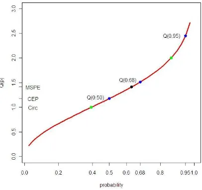
A robust and distribution free description of the measurement accuracy is obtained by reporting quantiles of the distribution of the absolute errors. For example, the 95% quantile means that 95% of the errors have a magnitude within the interval [0, Q(0.95)]. The remaining 5% of the errors can be of any value making the measure robust against up to 5% blunders. Another important measure is the 68.3% quantile of the absolute errors. It indicates the value where all differences smaller than this value amount to 68.3% of all errors. This percentage is also used to define the standard deviation (1·σ) at normal error distribution. The meaning of the robust accuracy measures can be explained by means of Figure 2 where the quantiles (Q) are plotted as function of the probability (p). Normal distribution of the errors is assumed and the unit of quantiles is the standard deviation.
If absolute values of the errors are used, Q(0.683) corresponds to 1·σ and Q(0.95) to 1.96·σ. The 50% quantile of the absolute values of the errors (red curve) equals to 0.67·σ and is named Median Absolute Deviation (MAD). Multiplication of MAD by the factor 1.4826 is then the Normalized Median Absolute Deviation (NMAD). At normal distribution the NMAD value corresponds to the standard deviation (1·σ). All of the robust
accuracy measures are summarized in Table 1. In the assessment of the horizontal accuracy, the assessment has first to be done for the single coordinate errors (ΔE, ΔN).
Figure 2. Robust accuracy measures: Median, Q(0.68), and Q(0.95). The quantile function Q(p) for absolute errors (red line) shows that Q(0.68) corresponds to 1·σ in case of normal distribution. When original errors are used (stippled black line) the difference dp=0.68 corresponds to the range of ±1·σ.
Median
(50% quantile)
Q
ˆ
x (0.5) = mx Normalized MedianAbsolute Deviation
NMAD=1.4826 mediani( |xi –mx|)
68.3% quantile
Q
ˆ
|x| (0.683) 95% quantileQ
ˆ
|x| (0.95) Table 1. Robust accuracy measures for a variable xAlso radial errors can be generated by
2 2
i i
i E N
r (1)
and then treated as absolute errors.
The confidence intervals (CI) of the accuracy measures have also to be calculated using a confidence level of 95%. For the robust accuracy measures the bootstrap method can be applied (Höhle&Höhle, 2009). The assessment of the horizontal accuracy has to be carried out by means of a sufficient number of checkpoints. They should be randomly distributed over the whole DTM area.
The planimetric errors can be visualized graphically together with an ellipse of constant probability, e.g. p=0.95. The parameters of the ellipse (semi axes and angle between major axis and Easting) are derived by means of formulae published in (Mikhail 1976). The centre of the ellipse has the coordinates µE and µN. The reduced radius (r’) is then:
(2)
Its distribution is derived from the joint (bivariate) distribution. There is a wish to characterize the planimetric error by a single value, for example by σr or σr’. Other suggestions derive
measures starting form the standard deviations of the two coordinate errors and the probability of a standard ellipse:
Mean Square Positional Error (MSPE)
2 2
N E
P
(3)
The MSPE is also named ‘point error’ and symbolized by σP. The probability that radial errors (ri) occur less than σP depends on the ratio σN/σE. If σE=σN the probability that ri < σP is p=0.632.
Circular Standard Error (σc)
This error is defined by 1.0·σc and p[ri < σc]=0.393. An approximation is obtained by
σc≈ 0.5·(σE+σN) (4)
Circular Error Probable (CEP)
The definition of CEP is p[ri<CEP]=0.5.
CEP0.50≈ 1.177 · σc = 0.589·(σE+σN) (5)
The calculation after formulae (4) and (5) are approximations and only valid when the relation σmin/σmax is not smaller than 0.6 (Congalton&Green, 2009). The CEP may be used with other probabilities, e.g. with p=0.95. Then the calculation is CEP0.95≈ 2.447·σc. The factor k=2.447 is derived from the χ2 – distribution with two degrees of freedom (cf. Figure 3).
In (Borre, 1990) the planimetric error is defined by:
2
2 2
' E N
P
(6)
In Figure 3 the mentioned accuracy measures may be compared with regard to their probability in the case σE=σN. Many different accuracy measures are not very useful and a selection has to be made. All mentioned accuracy measures will be used in the practical tests with the method of derived check points. A recommendation will be made which of the accuracy measures should be used in specifications and standards.
Figure 3. Horizontal accuracy measures and their probability
( ) 2
'
)
( i E 2 i N
In (ASPRS, 2005) and (Congalton & Green, 2009) the American standards for horizontal accuracy measures are described. These standards derive the standard deviation from the differences between the errors and the RMSE estimate (and not the Mean). A circular as well as an elliptical statistic is applied using RMSE values for the radius or coordinates respectively. A confidence interval on the estimate of RMSE is calculated at 95% probability. The NSSDA circular statistic, for example, corresponds to 1.731*RMSEr
4. A PROCEDURE FOR THE ASSESSMENT OF THE PLANIMETRIC ACCURACY
The use of houses is the base of the method proposed in (Höhle&Pedersen). Suitable houses are hip houses and cross gable houses (cf. Figure 1). The parameters of the planes are derived from laser footprints using robust adjustment. This means that observations of objects above or below the plane (e.g. chimneys, windows) are down-weighted and therefore have no influence on the results. Several iterations are carried out in order to find accurate solutions for the parameters of planes. Three adjacent planes are intersected to a point. For the intersected points the precision and confidence ellipses are derived and analyzed. Large and deformed ellipses will indicate a poor determination of the points. The derived spatial coordinates of these check points are compared with reference values derived by photogrammetry. A few ground control points are required in order to determine the exterior orientation data of the images. These six parameters may also be known from a preceding aerotriangulation. The well-defined checkpoints on top of the houses are manually measured. The achievable accuracy of this photogrammetric point determination when using modern digital cameras from an altitude of 1000m is a few centimetres. The images are also used to measure the corners of the roofs in order to extract all footprints inside a roof areal. The extraction of check points is carried out semi-automatically for a large area. If such houses do not exist the combination of gable houses can also be used. The derivation of the virtual checkpoints derived from ALS data can be done by the same procedure as for the hip houses. The reference values are determined by intersection of two lines measured by manual photogrammetry.
5. PRACTICAL TESTS
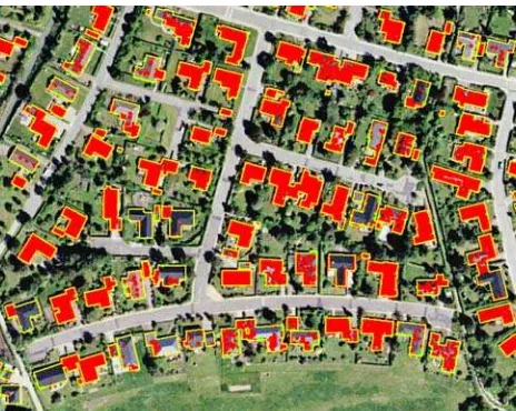
The practical tests for the determination of the planimetric accuracy of ALS data have been carried out with the original point cloud of the new Danish DEM. The data are collected by a Lite Mapper 5600 scanner produced by Riegel/IGI mbH. The average density of the point cloud was 0.45 points/m2 only. The overlap between strips was at least 5% of the swath width. The Inertial Measurement Unit (IMU) determined the attitude of the laser scanner with a nominal accuracy of 0.004° for roll and pitch angles. The footprint of the laser beam had a diameter of 0.5m. In the assessment of the horizontal accuracy some conditions have to be fulfilled. The roofs have to be plane with certain slope and containing more than four footprints. This condition has been checked by the programs. Additional data like orthoimages and maps helped in the selection of suitable houses (cf. Figure 4). The reference data and other roof points were derived from images taken by the large format digital frame camera DMC of Hexagon/Intergraph. The images had an overlap of 60% and a ground sampling distance of GSD=10cm.
The photogrammetric determination of reference data used four images.
Figure 4. Orthoimage and vector map are used to select suitable roofs. Note that not all of the roofs contain footprints (red areas)
The measuring of the image coordinates occurred on the screen
6. RESULTS
The analysis of the results will include the precision of the of a desktop computer. The same point had to be measured in two or more images. The exterior orientation of the aerial images was determined by bundle adjustment. Only four Ground Control Points (GCPs) were used. The processing was carried out by open-source software (IFP, 2009) running in a personal computer. The GCPs as well as a few checkpoints (for the determination of the quality of the orientation data) have been measured by means of GPS/RTK. The reference system was UTM with the coordinates Easting (E) and Northing (N). The orientation of the images proved to be very accurate. The standard deviation of the unit weight was 4.0µm in the image. The quality of the orientation was assessed by independent checkpoints. A RMSE of 4.2cm has been found for each of the two planimetric co-ordinates. It is assumed that the upper roof points have the same accuracy. Having such a high accuracy these measurements are qualified as reference data.
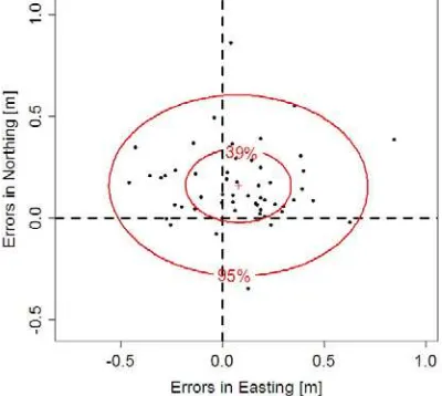
single coordinates and their 95% confidence intervals are contained in the lower part of Table 3. The Median is smaller than the Mean, the NMAD is smaller than the Standard Deviation and the Q|Δc|(0.683) is smaller than the RMSE. It means that the blunders have falsified the standard accuracy measures and their values are not correct.
igure 5. Coordinate errors together with the 95% and 39%
Easting [m] Northing [m]
F
confidence ellipses (bivariate normal)
MEAN 0.08
[0.01, 0.15] [0.11, 0.21] 0.16
Std. Dev.
[0.22, 0.32] [0.15, 0.22]
0.26 0.18
RMSE 0.27
[0.23, 0.33] [0.20, 0.30] 0.24
Median 0.07
[0.02, 0.18] [0.08, 0.19] 0.11
NMAD
[0.15, 0.34] [0.08, 0.18]
0.24 0.13
Q|Δc|(0.683) 0.26
[0.20, 0.31] [0.16, 0.29] 0.21
Table 3. the coord
order define the planimetric accuracy by one value instead
Standard r r’ Robust m
r [m]
r’ Accuracy
to
measures of inates.
In
of two, new variables, the radii ri and r’i, have been calculated for each point by formulae (1) and (2) and standard as well as robust accuracy measures have been derived (cf. Table 4). The robust accuracy measures (Median, NMAD) are again smaller than the standard accuracy measures (Mean, Std. Dev.). The Q(0.683)-values have about the same size as the RMSE values.
measures [m] [m] easures [m]
Mean 0.31 0.27 Median 0.28 0.24
Std. Dev. 0.18 0.17 NMAD 0.08 0.10 RMSE 0.36 0.31 Q(0.683) 0.36 0.32 1.731·RMSE 0.62 0.54 Q(0.950 0.64 0.56
Table c e he
ne value can also be derived from the standard deviations of the coordinates. These are approximations and the probability is
4. Ac uracy m asures of t radii
O
m] σP [m] σ’P [m]
NMAD=0.8496·median(|r
i-mr|) at bivariate distribution
changing with the relation σmin/σmax and is given for the special case σE = σN (cf. Table 5).
Probability CEP [
p=0.393 0.22 (=σc) 0.23 0.22
p=0.500 0.26 0.27 0.26 p=0.632 0.31 0.32 0.31
p=0.683 0.33 0.34 0.33 p=0.950 0.54 0.55 0.54
Tabl etric accuracy by one (probab or the case of ). The underlined values are the radii of the
es (cf. Table 5) are in good agreement with the quantiles of the unbiased radius (Q ) (cf. Table 4). The
e 5. Planim
σ =σ
value ility f
E N
standard circle (k=1.0)
The CEP- and σ’P–valu
r’
Mean Square Positional Error (MSPE=σP) is calculated by equation (3) with σP=32cm. Its exact probability is p=0.570 at the ratio σN /σE = 0.69. If this ratio is different, the probability will change, e.g. at σE /σN =1.0 to p=0.632. The better solution is, therefore, to derive quantiles with constant probability from the radial errors (r’i). The 95% quantile was determined with Qr’(0.95)=0.56m. In Figure 6 the accuracy measures based on the same probability (95%) are depicted and can, therefore, be compared.
0,5 0,54 0,58 0,62 0,66
1 2 3 4 5 6
[m
]
Figure 6. Planimetric errors with p=0.95. It means: 1=0.5(a+b), 2=CEP_0.95 (=NSSDA_elliptical statistic), 3=1.731*RMSE
rived from the semi-axes of the confidence ellipse nd the circular error probable (CEP_0.95) are smallest. The
SSION
The follow two topics, the used
method in
r (=NSSDA_circular statistic), 4=1.731*RMSEr’, 5=Qr(0.95), 6=Qr’(0.95)
The error de a
accuracy measures based on the radius (r) have higher values than the ones based on the unbiased radius (r’). Qr’ is nearly of the same size as the CEP_0.95.
7. DISCU ing discussion will comprise the
8. SUGGESTION OF A NEW STANDARD FOR PLANIMETRIC ACCURACY OF ALS
ta can be carried out using sloped roofs of houses. Well-defined
REFERENCES
ASPRS, 2005. Draft AS es: Horizontal Accuracy Reporting,
, pp. 385-396.
means of robust statistical methods, ISPRS Journal of
RS, 68(9), pp.
sity Press of America, New York.
chives of the
The National Su is thanked for
providing ALS data. C. Ø. Pedersen supported the author in combination of three gable houses is also possible. The
planarity of the roofs does not always exist. Objects above or below the plane have to be eliminated from the point cloud. The used robust adjustment eliminated such laser footprints. The sufficient number of footprints and inclination of the roofs will produce accurate check points. The plotting of confidence ellipses will disclose weak intersections. The assessment of the planimetric accuracy may in principle be combined with the assessment of the vertical accuracy. The accuracy of elevations derived by means of photogrammetry was not accurate enough in this test. Elevations of checkpoints on flat ground can accurately and easily be determined by means of geodetic measurements, e.g. by GNSS. The measurement of inclined roofs by means of GNSS is not very feasible. Imagery may not be available as in this case. However, the simultaneous acquisition of ALS and imagery will be more used in future than today. Most of the DEM applications require complete, reliable and interpreted elevations together with other data, which can be extracted from multi-spectral imagery. The event of new generations of digital aerial cameras will further improve the value of supplementing imagery. The accuracy measures to be applied have to take into account whether the distribution of the errors is normal or not normal. This was tested for the coordinates first. The chosen threshold for the absolute coordinate error (|Δci|≤3·RMSE) revealed one blunder at each coordinate. The values of the standard accuracy measures are, therefore, not correct. The plot of all errors together with confidence ellipses (cf. Figure 5) shows clearly that systematic shifts in the two coordinates exist and that three points are outside the 95% confidence ellipse. The use of the robust accuracy measures yields smaller values for the shifts in the coordinates (Median) and for the absolute deviations from the Median (NMAD). The Q|Δc|(0.683) is smaller than the RMSE. The confidence intervals for the Mean exceed 20% of the values. A higher number of checkpoints would have made the intervals smaller. The use of the 95% confidence ellipse is more appropriate than of the standard ellipse with a 39% confidence level only. The ellipse is defined by 3 values. The planimetric accuracy can be expressed by one value using either
σc,, CEP0.50, σP or σ’P as accuracy measure. The better solution is to derive quantiles of the radial errors (r’ and r’i) with a constant probability. Their values are robust against blunders and non-normal error distribution. The 95% quantile of the unbiased radial error (r’i) was determined with Qr’(0.95)=0.56m. The difference to Qr(0.95)=0.64m is relatively small. The size of planimetric error in the test is rather high; it is much higher than the vertical accuracy of ALS. The acquisition of a point cloud of higher density will not change the result very much. The improvement of the planimetric accuracy in ALS requires accurate system calibration and ground control. The checking of the planimetric accuracy is an important task of ALS projects.
The assessment of the planimetric accuracy of ALS da
checkpoints are derived from a large number of footprints covering three roof planes and intersecting the modelled planes to points. Accurate coordinates of these check points can be determined by means of photogrammetry. The errors in the coordinates have to be analyzed with respect to blunders and distribution. If the distribution of the errors is normal, the standard accuracy measures (Mean, Standard Deviation, and
RMSE) are applied for the coordinates and for the radii. In the case of non-normal distribution the robust accuracy measures have to be used. These are the Median, the NMAD for both coordinates and the 95% quantile of the unbiased radial error (Qr’(0.95)). All accuracy measures have to be supplemented by confidence intervals which will disclose whether the number of checkpoints were sufficiently high. A plot of all single errors together with a 95% confidence ellipse will display the overall geometric quality of the DEM.
PRS Lidar Guidelin
http://www.asprs.org/society/committees/standards/Horizontal_Accurac y_Reporting_for_Lidar_Data.pdf (accessed 1.4.2011)
Borre, K., 1990. Landmåling, ISBN 87-89088-24-7, Department of Planning, Aalborg University, Aalborg.
Congalton, R., Green, K., 2009. Assessing the Accuracy of Remotely Sensed Data, Taylor& Francis Group, Boca Raton.
Csanyi, N., Toth, C.K., 2007. Improvement of Lidar Data Accuracy Using Lidar-Specific Ground Targets, PE&RS, 73(4)
Fowler, A., Kadatskiy, V., 2011. Accuracy and Error Assessment of Terrestrial, Mobile and Airborne Lidar, Proceedings of ILMF, 10p.
IFP (2009). DGAP - Bundle Adjustment, http://www.ifp.uni-stuttgart.de/publications/software/openbundle/index.en.html (accessed 1.4.2011)
Höhle, J., Höhle, M., 2009. Accuracy assessment of digital elevation models by
Photogrammetry and Remote Sensing, 64 (2009), pp. 398-406.
Höhle, J., Pedersen, C.Ø., 2010, A new method for checking the planimetric accuracy of Digital Elevation Models data derived by airborne laser scanning, Proceedings of the Ninth International Symposium on Spatial Accuracy Assessment in Natural Resources and Environmental Sciences (“Accuracy 2010”), pp. 253-256.
Kager, H., 2004, Discrepancies between overlapping laserscanning strips – simultaneous fitting of laserscanner strips, International Archives of the Photogrammetry, Remote Sensing and Spatial Information Sciences, Commission III, WG III/1, 6p.
Maas, H.-G., 2002. Methods for Measuring Height and Planimetry Discrepancies in Airborne Laser Scanning Data. PE&
933-940.
Mikhail, E.M., 1976 Observations and Least Squares, ISBN 0-7002-2481-5, Univer
van der Sande, C., Soudarissanane, V., and Khoshelham, V., 2010Assessment of Relative Accuracy of AHN-2 Laser Scanning Data Using Planar Features, Sensors, 2010, 10, pp. 8198-8214.
Vosselman, G., 2008. Analysis of Planimetric Accuracy of Airborne Laser Scanning Surveys, pp. 99-104, International Ar
Photogrammetry, Remote Sensing and Spatial Information Sciences, Commission III, WG III/3.
ACKNOWLEDGEMENTS rvey and Cadastre of Denmark