AUTOMATIC DETECTION OF BUILDING POINTS FROM LIDAR AND DENSE IMAGE
MATCHING POINT CLOUDS
Evangelos Maltezos*, Charalabos Ioannidis
Laboratory of Photogrammetry, School of Rural and Surveying Engineering, National Technical University of Athens, Greece, Ε-mail: [email protected]; [email protected]
Commission III, WG III/2
KEY WORDS: LIDAR, point cloud, building extraction, scan line, filtering, change detection
ABSTRACT:
This study aims to detect automatically building points: (a) from LIDAR point cloud using simple techniques of filtering that enhance the geometric properties of each point, and (b) from a point cloud which is extracted applying dense image matching at high resolution colour-infrared (CIR) digital aerial imagery using the stereo method semi-global matching (SGM). At first step, the removal of the vegetation is carried out. At the LIDAR point cloud, two different methods are implemented and evaluated using initially the normals and the roughness values afterwards: (1) the proposed scan line smooth filtering and a thresholding process, and (2) a bilateral filtering and a thresholding process. For the case of the CIR point cloud, a variation of the normalized differential vegetation index (NDVI) is computed for the same purpose. Afterwards, the bare-earth is extracted using a morphological operator and removed from the rest scene so as to maintain the buildings points. The results of the extracted buildings applying each approach at an urban area in northern Greece are evaluated using an existing orthoimage as reference; also, the results are compared with the corresponding classified buildings extracted from two commercial software. Finally, in order to verify the utility and functionality of the extracted buildings points that achieved the best accuracy, the 3D models in terms of Level of Detail 1 (LoD 1) and a 3D building change detection process are indicatively performed on a sub-region of the overall scene.
* Corresponding author
1. INTRODUCTION
The technological development in the fields of computer vision and digital photogrammetry provides new tools and automated solutions for applications in urban studies, cadastre, etc, associated with urban development, identification of illegal constructions, 3D modelling, change detection, etc. Numerous algorithms have been developed over the years for the automatic building detection using LIDAR data and point clouds from dense image matching. Lodha et al. (2006) classified the whole scene into buildings, trees, roads, and grass applying several variations of Support Vector Machines (SVM). Using the features height, height variation, normal variation, LIDAR return intensity, and image intensity, they report an accuracy rate higher than 90%. Han et al. (2007) proposed a fast and memory-efficient segmentation algorithm similar to the region-growing and unsupervised-classification methods for airborne laser point clouds utilizing scan line characteristics. Zhou and Neumann, (2008) proposed an automatic algorithm which reconstructs building models from LIDAR data. After the removal of vegetation applying a SVM method based on local geometry property analysis, the planar roofs and the boundaries of buildings were extracted. Their classification algorithm achieved a success rate of 95%.
A different approach was proposed by Huang and Sester (2011) combining a bottom-up and a top-down approach to extract and refine building footprints from LIDAR data. Initially, a pre-segmentation step of the raster image of the point loud was conducted. Then, a 3D Hough Transform was chosen to detect the building points and an improved joint multiple-plane
detection was applied to find and label the LIDAR points on multiple roof facets. Finally, a top-down reconstruction was conducted via generative 3D models of buildings. Concerning the reconstruction of the building footprints, they achieved a success rate of about 90%. Lafarge and Mallet (2012) proposed a robust hybrid representation to create large-scale city models from 3D point clouds. The classification of the buildings was carried out implementing an energy minimization via a graph cuts based algorithm (Boykov et al., 2001) which included several geometric attributes such local non-planarity, elevation, scatter and regular grouping. Their algorithm was tested on LIDAR data as well as on a point cloud derived from Multi-View Stereo (MVS) imagery. Awrangjeb and Fraser (2013) presented a new robust rule-based segmentation technique for LIDAR point cloud data for automatic extraction of building roof planes using a data driven approach. Hu and Ye (2013) proposed a fast and simple algorithm based on scan line analysis using the Douglas-Peucker algorithm for the automatic detection of building points from LIDAR data. Sun and Salvaggio (2013) developed a fast and completely automated method to create watertight building models from airborne LIDAR point clouds. Concerning the building detection a robust graph cuts based method was used to segment vegetation from the rest of the scene content achieving an accuracy rate of 95.7%. Then, the ground terrain and building rooftop patches were extracted utilizing a hierarchical Euclidean clustering. Finally, a specifically designed region growing algorithm with smoothness constraint was applied using the point normals and their curvatures. Also, alternative approaches combining the advantages of both LIDAR and multispectral images have been applied (Liao and Huang, 2012). Hron and Halounova (2015)
focused on point clouds that derived from digital aerial images using derived layers that contained additional information about the road and railway networks, shadow and vegetation/NDVI masks, etc.
However, interesting studies have been implemented that focused on feature enhancement at LIDAR point clouds (Duguet et al., 2004; Daniels et al., 2007; Gao and Neumann, 2014). Since LIDAR point clouds often suffer from noise and local under-sampling, filtering techniques could be implemented to enhance the geometric properties of each point and therefore the appearance of the object of interest. The quality (i.e., density, presence of transparent materials, etc) of the raw LIDAR point cloud may has a significant effect to each point cloud classification. Simple and efficient algorithms for the classification of point clouds, which constitute a very large amount of data, are required towards the challenge of the increasingly greater demands for accurate and real-time classification applications.
This paper exploits the use of the geometry of the surface which is derived from the normal vector estimation using the value of component Nz, in combination with filtering techniques to any post-processing. Furthermore, it does not involve training data. In this context, a simple, easy to implement and efficient approach of scan line smooth filtering is proposed as well as a bilateral filter is implemented and evaluated.
2. PROPOSED APPROACHES FOR THE AUTOMATIC DETECTION OF BUILDING POINTS
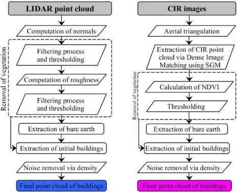
In this study, the point clouds of buildings of an urban area are automatically extracted using two different types of data. The first type of data is a LIDAR point cloud with a point density of 40 cm; the second type of data is a dense point cloud which extracted by dense image matching using the stereo SGM method (Hirschmüller, 2008) from high resolution CIR digital aerial imagery with a ground sample distance (GSD) of 20 cm. Figure 1 illustrates the flow chart of the proposed approaches.
Figure 1. Workflow of the automatic detection of building points from the LIDAR point cloud (left) and the CIR point cloud (right).
The first step of the applied procedures is the removal of the vegetation (dashed rectangles in Figure 1). At the LIDAR point cloud two different methods are implemented and evaluated using the normal and the roughness values:
- the proposed scan line smooth filtering and a thresholding process, and
- a bilateral filtering and a thresholding process.
On the other hand, the CIR point cloud embodies the multispectral information and so a variation of the NDVI (named NDVI in the rest of the paper) is calculated to separate the vegetation.
In the second step, an approach similar to Kilian et al. (1996) is conducted to extract the bare earth based on a morphological operator along the scan line of the point cloud. In the third step, the results of the previous two steps are utilized to extract the point clouds of the initial buildings. At the fourth step the density of the remaining points is examined in a search area and thus isolated points or tiny blobs of points are removed. In the fifth step, the final point cloud of buildings of each approach is extracted. The implementation and the evaluation of the proposed approaches is made using the MATLAB computing environment as well as the open-source project CloudCompare (Girardeau-Montaut, 2015) and the LAStools and ERDAS IMAGINE commercial software packages. includes buildings with complex structure, the normals were estimated applying a local model of 2D triangulation for the optimum adaptation at the building’s surface (instead of using a local model of a plane or a height function which requires a radius of a local neighborhood) using the CloudCompare software. The normal value of Nz tends to the value 1, where 1 is the max value, in case of a planar surface (in the field, usually located within to the range 0.85 to 1). Since some rooftops are rough or irregular due to the presence of complex sloping roofs, chimneys, solar water heaters, etc, the Nz value deviates significantly from the value 1. Similarly, vegetation, which in majority present disorderly dispersion of the value Nz (having significantly different Nz values from the value 1), may present Nz values close enough to the value 1 in cases of vegetation with very flat canopies; for example, dense arrays of trees or foliages. Considering the above, an active filtering is quite capable to enhance the correct entries (Nz value close to the value 1 for building rooftops and Nz value far from the value 1 for vegetation) and to absorb simultaneously incorrect entries (Nz value close to the value 1 for vegetation and Nz value far from the value 1 for building rooftops).
A simple and easy to implement filtering approach is conducted along the scan line of the LIDAR point cloud calculating the average of the Nz values within a defined neighbourhood symmetrically from a center point. The new calculated Nznew
value for each point is computed as:
i
where pi is a position of a set of 3D points
31 2 N i
P= p ,p ,...,p ,p R and k is the number of the symmetric
points of the neighborhood plus the center point p. Equation (1) is performed to each point to include retrospectively the Nznew
value of each previous point. Thus, a powerful filtering is carried out; the larger the neighbourhood the more intense is the effect of filtering. In this sense, an excessive filtering may cause false entries and therefore to deform the boundaries of buildings. Hence, in this study, a small neighbourhood was selected including 3 points (the center point, its previous and its next point). After the filtering of the Nz values, a thresholding process is carried out removing the points that represent the vegetation whose Nz values where lower than 0.85 as well as possible facade building points. In a second phase, a further process is conducted to eliminate few cases of possible remaining vegetation. Firstly, the feature roughness is calculated on the thresholded point cloud of the previous step. Then, the roughness values are imported at Equation (1) using a neighbourhood of 3 points to absorb local cases of intense roughness on planar surfaces and simultaneously to highlight possible remaining vegetation. In general, using only the roughness as criterion of the classification of a point cloud may cause false classifications especially on dense vegetation, complex sloping roofs, small extensions of major buildings, etc. Since this study aims to detect even small buildings (of an area as small as 5 m2), the use of roughness obtained into consideration only complementary, and optionally if needed, using strict criteria such as the calculation of roughness in a search area of 1 m and the removal of points whose roughness values are higher than 0.10 m.
Furthermore, the same procedure was carried out implementing a bilateral filter which originally proposed in image processing (Smith and Brady, 1997; Tomasi and Manduchi 1998). The bilateral filter is a non-iterative and simple non-linear filter which efficiently filters and smooths the values of the quantity of interest. The output value is a weighted average of the input value based on the spatial distance of neighbours and on the influence difference that penalizes values across features (Gao and Neumann, 2014). Extensions of the bilateral filter could be found in the literature (Fleishman et al., 2003; Jones et al., 2003). The parameters of the filtering of the Nz values that finally selected associated with the best results were spatial sigma = 3.05 and scalar sigma = 0.35. A thresholding process at the filtered Nz values is carried out removing vegetation points whose Nz values are lower than 0.85 as well as possible facade building points. Also, the bilateral filter is implemented to roughness values to eliminate possible remaining vegetation. The same strict criteria concerning the use of roughness applied using a more intense filtering step with spatial sigma = 1 and scalar sigma = 1. Figure 2 shows the effect of the scan line smooth filtering and the bilateral filtering of the Nz values compared to the initial Nz values. Figure 3 illustrates a part of the scene of the final cleared from vegetation LIDAR point clouds.
2.1.2 Semi-global matching and removal of vegetation calculating the NDVI at the CIR point cloud: SGM is an efficient, detailed, accurate and reliable stereo method for image based 3D surface reconstruction (Haala, 2011). The global energy E(D) is defined as:
(2)
Figure 2. The LIDAR point cloud coloured by the initial Nz values (top); the filtered Nz values by the bilateral (middle) and the scan line smooth filtering (bottom).
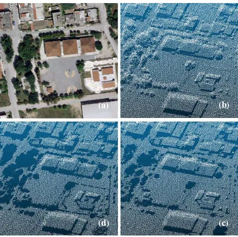
Figure 3. Removal of the vegetation of the LIDAR point clouds; (a) the orthoimage (b) the raw LIDAR point cloud, (c) the cleared LIDAR point cloud by the bilateral filtering, and (d) the cleared LIDAR point cloud by the scan line smooth filtering.
(b) (a)
(c) (d)
The first term is the sum of a pixel-wise matching cost for all pixels p at their disparities Dp. The proposed algorithm based initially at matching cost function Mutual Information (MI). However, variations of this algorithm may be implemented using other matching cost functions (Hirschmüller and
Scharstein, 2009). The second term adds a constant penalty P1 for all pixels q in the neighborhood Np of p, for which the disparity differences are small (i.e., 1 pixel). The third term penalizes larger disparity differences (i.e., independent of their size) with a larger constant penalty P2. Lower penalties allow an adaptation to slanted or curved surfaces whereas larger penalties have to do with discontinuities. Since discontinuities are often visible as intensity changes, an adaptation of P2 to the intensity gradient for neighborhood pixels p and q in the reference image Ib is carried out by: (should be 16 for providing a good coverage of the 2D image), towards each pixel of interest using dynamic programming. For each pixel and disparity, the costs of all paths are summed and then the disparity is determined using the Winner Takes All considered satisfactory and suitable for the area of interest as an optimal combination of focal length, image scale, overlap of images and base to height ratio was accomplished.
The near-infrared (NIR) channel is a very good source of information for the detection of vegetation. Since this colour channel is much more important than the blue channel, aerial images were prepared in false colours, created with the combination of near-infrared, red and green channels (Hron and Halounova, 2015). Noted, that in case of lack of NIR channel, machine learning techniques could be used to detect vegetation. For the case of CIR point cloud, a filtering process as described in section 2.1.1 seems that is not feasible due to the rough surface and not accurately shaped building’s outlines of the dense image matching point clouds.
In this study, a dense point cloud from CIR images was extracted. First, an aerial triangulation of the stereo-pair of the CIR digital aerial imagery is performed using 6 Ground Control Points (GCPs). Then, the SGM method is implemented using the ERDAS IMAGINE package. Instead of generating an image mask of the vegetation, the NDVI is calculated directly to the CIR point cloud using the channels where the vegetation is fully and dimly depicted. Thus, a vegetation index is calculated which takes negative values for vegetation areas and positive values for the rest. Therefore, the NDVI threshold was selected as 0 to remove the vegetation. Figures 4-top and 4-bottom depict a part of the scene of the CIR point cloud and the cleared corresponding after thresholding the NDVI respectively.
The next step of the proposed approach is the extraction of the bare earth from each point cloud of the sections 2.1.1 and 2.1.2. Since the urban scenes rarely present intense topographic ground surface, the bare earth may detected based on a morphological operator similar to Kilian et al. (1996) selecting the deepest point inside a window of a certain size. The window is moved by a certain step along the scan line at each point cloud associated with the size of the maximum building. The size of the window of the operator varies depending on the scene so as to avoid false ground detection. As the morphological operator is implemented at the cleared from vegetation point clouds, a safe extraction of bare earth is conducted avoiding false ground detection caused by long arrays of trees or low vegetation.
The only parameter involved in this step is the size of the maximum building. This size can be determined either by a visual inspection of the point cloud or by an automatic process (e.g., a pre-segmentation). In this study the size of the maximum building is equal to 120 m due to the existence of industrial buildings in the area. To obtain an integrated and comprehensive point cloud of the bare earth, a densification process via meshing and resampling with a similar point density of the initial corresponding point cloud is carried out. Finally, the point clouds of the buildings (with height larger than 2.5 m) are extracted using the point clouds of the sections 2.1.1 and 2.1.2 and the corresponding bare earth point clouds that extracted in this section.
2.3 Noise removal and extraction of the final point cloud of buildings
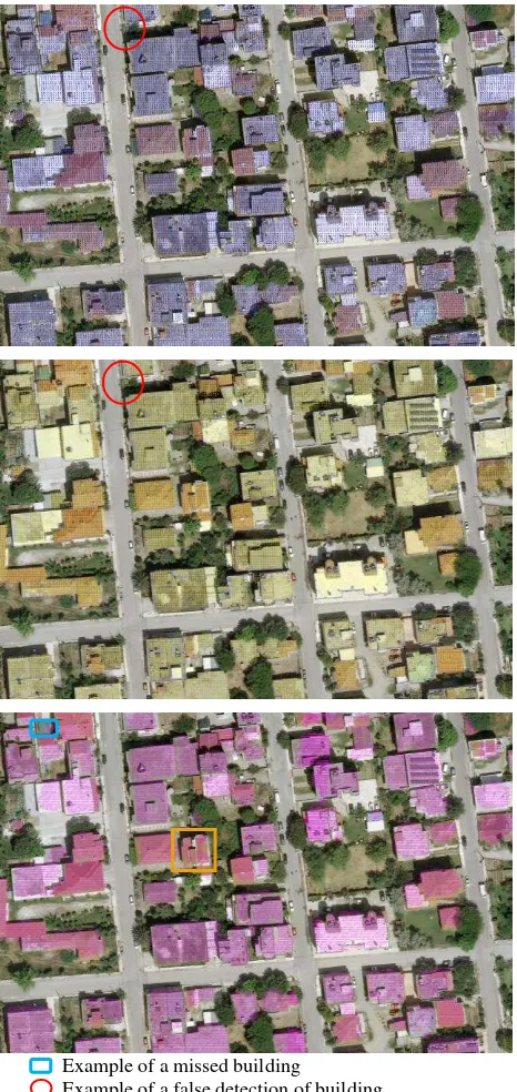
In the final step of the proposed procedure, possible remaining isolated points or tiny blobs of points with small number of neighbours (less than 20 for the LIDAR point cloud and less than 55 for the CIR point cloud) are removed using a search area with a radius of 2 m. Figure 5 depicts representative results of the final point clouds of buildings using the proposed approaches for a part of the scene that is superimposed on an existing orthoimage.
Example of a missed building Example of a false detection of building
Example of a poor performance of a detected building Figure 5. Final point cloud of buildings superimposed on an
orthoimage, using the bilateral filtering approach coloured in blue (top) and the scan line smooth filtering approach coloured in yellow (middle) at the LIDAR point cloud; the CIR point cloud from SGM coloured in magenta (bottom).
For comparison reasons, a classification process utilizing the LIDAR point cloud is implemented using the software packages of LAStools (lasground_new, lasheight and lasclassify) and ERDAS IMAGINE whose results are depicted in Figure 6. Several combinations of parameters were tested for the classification process of the LAStools including search area with a size of 1 m, 2 m, 3 m, 4 m and 5 m with the following combinations of building planarity and forest ruggedness: 0.1 m / 0.2 m, 0.1 m / 0.3 m, 0.1 m / 0.4 m, 0.1 m / 0.5 m, 0.2 m / 0.4 m and 0.3 m / 0.6 m. The best result was observed using a
search area of 5 m and a combination of building planarity and forest ruggedness of 0.3 m and 0.6 m respectively.
The parameters of the ERDAS IMAGINE that finally selected associated with the best results were:
Min slope = 30 deg, Min area = 5 m2, Min height = 2.5 m, Max area = 1400 m2, Plane offset = 0.3 m, Roughness = 0.6 m, Max height for low vegetation = 2 m,
Min height for high vegetation = 5 m.
Also, several combinations of parameters were tested, e.g., the Plane offset and Roughness took values: 0.2 m / 0.5 m or 0.1 m / 0.4 m or 0.3 m/ 0.5 m.
Example of a false detection of building
Figure 6. Final point cloud of buildings superimposed on an orthoimage, using the classification process in LAStools coloured in green (top); the classification process in ERDAS IMAGINE coloured in cyan (bottom) using the LIDAR point cloud.
3. EVALUATION OF THE RESULTS
The application area is a small town near Thessaloniki, in northern Greece, at an area of 0.33 Km2 containing 501 industrial and residential buildings. The type of vegetation of the scene is characterized as moderate. However, long arrays or groups of dense trees between the buildings, high vegetation beside the boundary of buildings as well as buildings surrounded or occluded by high trees exist. This situation in combination with the complex building structure with sloping roofs, chimneys, solar water heaters, small extensions or additions of major buildings, etc, constitutes a challenge towards an accurate and reliable automatic building detection process. To quantitatively evaluate the proposed approaches, the success rates of completeness, correctness and quality are used. According to the ISPRS guidelines (Rutzinger et al., 2009):
TP Completeness=
TP FN (4)
TP Correctness=
TP FP (5)
Quality= TP
TP FP FN (6)
where TP, FP, and FN denote true positives, false positives, and false negatives, respectively. Table 1 depicts the evaluation of the building results.
Approach Completeness Correctness Quality Scan line
smooth filtering
97.6% 98.2% 95.9%
Bilateral
filtering 99.8% 96.0% 95.8%
CIR point
cloud 93.0% 91.6% 85.7%
LAStools 92.0% 79.2% 74.1%
ERDAS
IMAGINE 99.0% 84.1% 83.4%
Table 1. Evaluation of the automatic detection of building points results.
The scan line smooth filtering and the bilateral filtering approaches achieved similar quality success rate. However, the scan line smooth filtering approach presented greater correctness but less completeness than bilateral filtering approach due to its powerful filtering. Thus, although the vegetation was almost completely removed, local complex cases of small extensions or additions of buildings (which were described partly due to the available density of the LIDAR point cloud) were incorrectly removed increasing the FN. Conversely, the bilateral filtering approach implements a more gently filtering and for this reason presents reverse performance on the rates of correctness and completeness presenting more FP associated with cases of dense and high trees. Although the scan line smooth filtering approach requires only the definition of the number of the symmetric points of the neighborhood, optimal results using the same value of k for the filtering of the Nz and roughness values were achieved. This is a comparative advantage to the bilateral filtering approach as the parameters of spatial sigma and scalar sigma were differently tuned to achieve the optimal results.
On the other hand, point clouds that had been extracted by dense image matching techniques suffer from other problems such occlusions, complex scenes, radiometric differences, texture-less areas, etc. Thus, although the higher density of the CIR point cloud and the use of the NDVI which removed the vegetation completely, FN and FP were observed mainly due to mismatches at complex cases of small buildings and unstable interpolations respectively.
Concerning the commercial software, the success rate of quality of the LAStools is low mainly due to several false detections associated with the vegetation. Unlike the LAStools, the ERDAS IMAGINE enables takes into account more parameters for the point classification process and therefore yielded higher success rates.
4. EXPLOITATION OF THE PROPOSED APPROACHES
The successful detection of the building points from a LIDAR or a dense image matching point cloud using the proposed approaches may be used on several applications, such as the creation of 3D city models, the building change detection using multi temporal data sets, etc. Indicative examples of these applications are developed in the following sections to verify the accuracy and reliability which may be achieved as well as the utility and functionality of the proposed approaches.
4.1 3D modelling
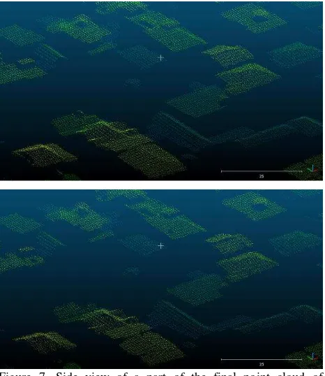
Using a visual inspection and superimposition at the raw LIDAR point cloud was approved that the final buildings that extracted via the bilateral filtering and the scan line smooth filtering approach have the proper density and fidelity to be used as input at several algorithms for 3D modelling in terms of LoD 1 or LoD 2 (Figure 7). In LoD 1 buildings are represented as block models (usually extruded footprints) and LoD 2 are building models with roof structures and textures, as defined by CityGML which is an open data model and XML-based format for the storage and exchange of virtual 3D city models (http://www.citygml.org/).
Figure 7. Side view of a part of the final point cloud of buildings coloured by the point height, using the bilateral filtering approach (top) and the scan line smooth filtering approach (bottom).
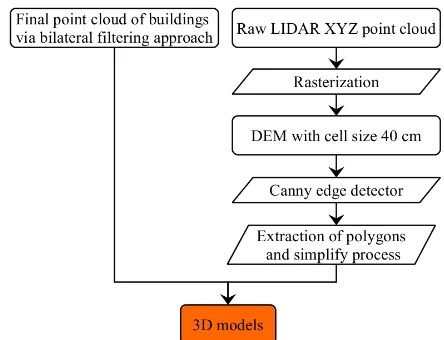
A simple and quick process is proposed to create the 3D models of the buildings that extracted by the bilateral filtering approach (which presented slightly sharper edges of buildings compared to the point cloud that extracted via the scan line smooth filtering) in terms of LoD 1. Figure 8 shows the proposed workflow which utilizes the results of a sub-region of the overall scene of the bilateral filtering approach and a corresponding edge map.
Figure 8. Workflow of the creation of the 3D models in terms of LoD 1.
The creation of a 3D building model is a demanding task since sharp and clear boundaries are required to describe the buildings. The combined use of an edge map is neseccary to absorb possible distortions of the boundaries of the extracted point cloud of buildings or small point gaps due to the thresholding process. In the described application an edge map was extracted through the implementation of the Canny edge detector (Canny, 1986) on the Digital Elevation Model (DEM) of the raw LIDAR point cloud. The best tuning of the parameters of the Canny edge detector to minimize insignificant edges was applied. A DEM cell size of 40 cm (which is the cell size of the edge map too) was selected in order to fully exploit the raw LIDAR point cloud. Figure 9 illustrates the results of the aforementioned workfow.
Figure 9. Top left: the DEM of the raw LIDAR point cloud data with a cell size of 40 cm; Bottom left: the corresponding edge map; Right: the extracted 3D models of buildings in terms of LoD 1 superimposed on an orthoimage.
4.2 3D building change detection
A 3D building change detection process is carried out at the same sub-region of section 4.1 using the final point cloud of buildings that extracted via the bilateral filtering approach (named “epoch 2”). A DEM with a cell size of 40 cm is extracted, and transformed to a point cloud (named “epoch 1”), using existing 3D vectors that included in a GIS database of a previous period. Then, the Multiscale Model to Model Cloud Comparison (M3C2) algorithm by Lague et al. (2013) between the point clouds of “epoch 1” and “epoch 2” was implemented.
Figure 10. The 3D building change detection results. Building points coloured in grey depicts the new buildings and (sighed by yellow ellipses).
Figure 10 shows the result of the 3D building change detection process. Points coloured in grey depict building points of the “epoch 2” for which no homologous points were found at “epoch 1”. These points indicate the new buildings. Noted, that these points can be separated and superimposed at existing true-orthoimages, topographic charts, etc. Also, possible height additions of buildings that remain horizontally unchanged are examined. The height difference between homologous points of the unchanged buildings of the two epochs was calculated using as significant height difference a height threshold of 3 m associated with the height of a typical floor. In the sub-region depicted in Figure 10 no height additions of buildings were observed as the vast majority of the height differences were less than the height threshold of 3 m.
5. CONCLUSIONS
This study aims to automatically detect building points: (a) from LIDAR data using simple techniques of filtering that enhance the geometric properties of each point, and (b) from a CIR dense image point cloud that extracted using the SGM technique. The proposed approaches are considered to be satisfactory; especially those that implement the proposed scan line smooth filtering and the bilateral filtering at the LIDAR point cloud as success rates of completeness, correctness and quality larger than 95% are achieved without the use of training data or any additional information, such as intensity or multiple returns. In comparison, high success rates of completeness (larger than 90%) but relatively low success rates of correctness are achieved using the commercial packages of LAStools and ERDAS IMAGINE. This shows the need of more robust techniques (not based mainly on roughness) to decrease false positive entries on complex scenes with dense and high vegetation.
The results of the proposed approaches on 3D modeling and 3D building change detection ensure that the extracted final point clouds via the filtering techniques can be used for urban planning, cadastral applications, etc. In addition, point clouds that derived from high resolution CIR digital aerial imagery have great potential as satisfactory success rates are achieved. However, more sophisticated point cloud classification techniques will be used in future work to optimize the results.
ACKNOWLEDGEMENTS
This research was conducted in the framework of the research project “5 Dimensional Multi-Purpose Land Information System” (5DMuPLIS). For the Greek side 5DMuPLIS project is
co-funded by the EU (European Regional Development Fund/ERDF) and the General Secretariat for Research and Technology (GSRT) under the framework of the Operational Program "Competitiveness and Entrepreneurship", "Greece-Israel Bilateral R&T Cooperation 2013-2015". Also, the authors would like to thank the Geosystems Hellas for providing the LIDAR data and the CIR images.
REFERENCES
Awrangjeb, M., Fraser, C.S., 2013. Rule-based segmentation of LIDAR point cloud for automatic extraction of building roof planes. In:City Models, Roads and Traffic (CMRT 2013), pp.1-6
Boykov, Y., Veksler, O., Zabih, R., 2001. Fast approximate energy minimization via graph cuts. PAMI, 23(11).
Canny, J., 1986. A computational approach to edge detection.
IEEE Trans. Pattern Analysis and Machine Intelligence, 8, pp. 679-698.
Daniels, J.I., Ha, L.K., Ochotta, T., Silva, C.T., 2007. Robust smooth feature extraction from point clouds. In: Proceedings of the IEEE International Conference on Shape Modeling International 2007, Washington, USA, pp. 123-136.
Duguet, F., Durand, F., Drettakis, G., 2004. Robust Higher-Order Filtering of Points. Technical Report RR-5165, INRIA.
Fleishman, S., Drori, I., Cohen-Or, D., 2003. Bilateral mesh denoising. In: ACM SIGGRAPH 2003 Papers, New York, USA, pp. 950-953.
Gao, Z., Neumann, U., 2014. Feature enhancing aerial LiDAR point cloud refinement. In: Three-Dimensional Image Processing, Measurement (3DIPM), and Applications 2014, SPIE, Vol. 9013.
Girardeau-Montaut, D., 2015. CloudCompare - Open Source Project. http://www.danielgm.net/cc/
Haala, N., 2011. Multiray Photogrammetry and Dense Image Matching. In: Photogrammetric Week '11, Ed. D. Fritsch, Wichmann, Berlin/Offenbach, pp. 185-195.
Han, S. H., Lee, J. H., Yu, K.Y., 2007. An Approach for Segmentation of Airborne Laser Point Clouds Utilizing Scan-Line Characteristics. ETRI Journal, 29, pp. 641-648.
Hirschmüller, H., 2008. Stereo processing by semi-global matching and mutual information. In: IEEE Transactions on Pattern Analysis and Machine Intelligence, 30(2), pp. 328-41.
Hirschmüller, H., Scharstein, D., 2009. Evaluation of stereo
matching costs on images with radiometric differences. In:
IEEE Transactions on Pattern Analysis and Machine Intelligence, 31(9), pp. 1582-1599.
Hron, V., Halounova, L., 2015. Use of aerial images for regular updates of buildings in the fundamental base of geographic data of the Czech republic. In: International Archives of the Photogrammetry, Remote Sensing and Spatial Information Sciences, Munich, Germany, Vol. XL-3/W2, pp-73-79.
Hu, X., Ye, L., 2013. A fast and simple method of building detection from LiDAR data based on scan line analysis. In:
ISPRS Annals of the Photogrammetry, Remote Sensing and Spatial Information Sciences, Regina, Canada, Vol. II-3/W1, pp. 7-13.
Huang, H., Sester, M., 2011. A hybrid approach to extraction and refinement of building footprints from airborne data. In:
International Archives of the Photogrammetry, Remote Sensing and Spatial Information Sciences, Guilin, China, Vol. XXXVIII-4/W25, pp. 153-158.
Jones, T.R., Durand, F., Desbrun, M., 2003. Non-iterative, feature-preserving mesh smoothing. In: ACM SIGGRAPH 2003 Papers, New York, USA, pp. 943-949.
Kilian, J., Haala, N., Englich, M., 1996. Capture and Evaluation of Airborne Laser Scanner Data. In: International Archives of Photogrammetry and Remote Sensing, Vol. XXXI, Part B3, pp. 383-388.
Lafarge, F., Mallet, C., 2012. Creating large-scale city models from 3D-point clouds: A robust approach with hybrid representation. Int. J. Computer Vision, pp. 1-17.
Lague, D., Brodu, N., Leroux, J., 2013. Accurate 3D comparison of complex topography with terrestrial laser scanner: application to the Rangitikei canyon (N-Z). ISPRS Journal of Photogrammetry and Remote Sensing, 82, 10-26.
Liao, C., Huang, H., 2012. Classification by using multispectral point cloud data. In: International Archives of the Photogrammetry, Remote Sensing and Spatial Information Sciences, Melbourne, Australia, Vol. XXXIX-B3, pp. 137-141.
Lodha, S.K., Kreps, E.J., Helmbold, D.P., Fitzpatrick, D., 2006. Aerial LIDAR data Classification using support vector machines (SVM). In: Proceedings of the International Symposium on 3D Data Processing, Visualization, and Transmission, Chapel Hill, NC, pp. 567–574.
Rutzinger, M., Rottensteiner, F., Pfeifer, N., 2009. A comparison of evaluation techniques for building extraction from airborne laser scanning. IEEE Journal of Selected Topics in Applied Earth Observations and Remote Sensing, 2(1), pp. 11-20.
Smith, S.M., Brady, J.M., 1997. Susan - a new approach to low level image processing. International Journal of Computer Vision, 23 (1), pp. 45-78.
Sun, S., Salvaggio, C., 2013. Aerial 3D building detection and modeling from airborne LiDAR point clouds. IEEE Journal of Selected Topics in Applied Earth Observations and Remote Sensing, 6(3), pp. 1440-1449.
Tomasi, C., Manduchi, R., 1998. Bilateral Filtering for gray and color images. In: Proceeding of the IEEE International Conference on Computer Vision, Bombay, India, pp.839-846.
Zhou, Q., Neumann, U., 2008. Fast and extensible building modelling from airborne lidar data. In: Proceedings of the 16th ACM SIGSPATIAL International Conference on Advances in Geographic Information Systems, New York, USA, pp. 7:1–7:8.