HIERARCHICAL HIGHER ORDER CRF FOR THE CLASSIFICATION OF AIRBORNE
LIDAR POINT CLOUDS IN URBAN AREAS
J. Niemeyera,∗, F. Rottensteinera, U. Soergelb, C. Heipkea
a
Institute of Photogrammetry and GeoInformation, Leibniz Universit¨at Hannover, Germany -(niemeyer, rottensteiner, heipke)@ipi.uni-hannover.de
b
Institute for Photogrammetry, University of Stuttgart, Germany [email protected]
Commission III, WG III/4
KEY WORDS:Classification, Point Cloud, Higher Order Random Fields, Contextual, Lidar, Urban
ABSTRACT:
We propose a novel hierarchical approach for the classification of airborne 3D lidar points. Spatial and semantic context is incorporated via a two-layer Conditional Random Field (CRF). The first layer operates on a point level and utilises higher order cliques. Segments are generated from the labelling obtained in this way. They are the entities of the second layer, which incorporates larger scale context. The classification result of the segments is introduced as an energy term for the next iteration of the point-based layer. This framework iterates and mutually propagates context to improve the classification results. Potentially wrong decisions can be revised at later stages. The output is a labelled point cloud as well as segments roughly corresponding to object instances. Moreover, we present two new contextual features for the segment classification: thedistanceand theorientation of a segment with respect to the closest road. It is shown that the classification benefits from these features. In our experiments the hierarchical framework improve the overall accuracies by 2.3 % on a point-based level and by 3.0 % on a segment-based level, respectively, compared to a purely point-based classification.
1. INTRODUCTION
1.1 Motivation
The automatic interpretation of airborne lidar point clouds in ur-ban scenes is an ongoing field of research. Usually, one of the first steps for inferring semantics is a point cloud classification. In computer vision and remote sensing it was shown that contextual knowledge can be used to improve classification results (Gould et al., 2008; Schindler, 2012). Conditional Random Fields (CRF) offer a flexible framework for the integration of spatial relations. However, in most related approaches this context is limited to a small local neighbourhood due to computational restrictions. Hence, they do not exploit the full potential of CRF. Operating on segments instead of points is one possibility to integrate more spatial information. Nevertheless, for example Shapovalov et al. (2010) showed that this leads to a loss of 1-3 % in overall accu-racy in their experiments compared to a point-based classification due to generalisation errors. A trade-off is the use of a Robust Pn
Potts model (Kohli et al., 2009), which considers higher or-der cliques. This model favours the members of a clique to take the same label but also allows for a few members assigned to other classes. This ‘soft‘ segmentation preserves small details in a better way compared to standard segmentation methods. How-ever, interactions between the cliques can not be considered in this model.
The aim of our work is to integrate long range interactions while still preserving small structures in the scene classification. We develop a hierarchical framework consisting of two layers, which considers a supervised contextual classification on a point layer as well as on a segment layer via CRF. In order to avoid generalisa-tion errors, the segments are generated in each iterageneralisa-tion based on the results of the point-based classification, and hence they corre-spond more and more closely to the objects. In this way the ad-vantages of operating on both levels of detail are combined. Our
∗Corresponding author
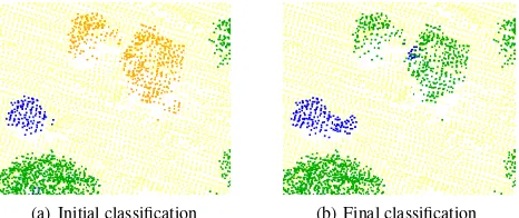
(a) Initial classification (b) Final classification
Figure 1. Example of a correction of our framework. The two trees in the center of 1(a) are wrongly labelled asbuilding (or-ange) in the initial point-based classification. After iterating through the two CRF layers several times, these points are cor-rectly classified astreethanks to context information (1(b)).
iterative procedure enables the correction of potentially wrong decisions at a later stage. Figure 1 shows an example of label hy-pothesis revision: In a first point-based classification, visualised in Fig. 1(a), the two trees in the centre were wrongly assigned to classbuilding(orange). The integration of context in a larger spatial scale as well as the adoption of the segments in our itera-tive method lead to an elimination of these errors, and hence to a correct labelling of these points astree(green) (Fig. 1(b)).
Additionally, we suggest two new contextual features for the clas-sification of airborne lidar point clouds. They describe the rela-tive position and orientation of segments in the scene, and help to further increase the overall accuracy of the classification.
1.2 Related work
or-der CRF, and the integration of contextual features. Of course, these combinations have also been combined.
The first group are thehierarchical models. Xiong et al. (2011) showed how point-based and region-based classification of lidar data can interact in a pairwise CRF. They proposed a hierarchi-cal sequence of relatively simple classifiers that are applied to segments and points. Starting either with an independent clas-sification of points or segments, in subsequent steps the output of the previous step is used to define context features that help to improve the classification results. In each classification stage, the results of the previous stage are taken as input. This work inspired our methodology. However, we exploit more complex interactions between the objects. Albert et al. (2015) also tackle the challenge of classifying data considering two scales of con-text. Their application is image classification of land cover (on a superpixel level) and the update of land use objects (on a higher semantical level). Similar to our approach they chose a hierar-chical CRF. The major difference is that in our case the object boundaries are not constant, which makes the task more difficult because in addition a good segmentation has to be found.
A further option to consider regional context in the classification process is the use ofhigher order CRF. We restrict this discus-sion to the work with point clouds. Kim et al. (2013) introduce a Voxel-CRF framework for jointly estimating the semantic and geometric structure of an indoor RGB-D point cloud for robotic navigation applications. The authors used an associative higher-order model based on Hough voting and categorical object detec-tion with the aim of identifying voxels belonging to the same ob-ject. Sengupta and Sturgess (2015) have a similar goal. They per-formed object detection and reconstruction from stereo images, also operating in voxel space. Both approaches classify voxels of a fixed size. In contrast, we make use of iteratively adapting seg-ments. These segments are generated with the RobustPn
Potts model (Kohli et al., 2009), which is more flexible and leads to a ‘soft‘ segmentation. This model favours the members of a clique to be assigned to the same class label. However, members can have a different label. The degree of penalisation depends on the ratio of those members to the total number of clique members. For this reason, it allows for some inhomogeneity, which may preserve small details in the scene. The cliques are generated in advance, for example by a segmentation algorithm. Also multiple segmentations with potentially overlapping segments can be used (Kohli et al., 2009). This enables the consideration of multiple spatial scales. However, interactions between the cliques can not be modelled by RobustPnPotts models; the expressive power is still restricted.
Najafi et al. (2014) set up a non-associative variant of CRF for point clouds. They first performed a segmentation and then ap-plied the CRF to the segments. Overlapping segments in 2D are considered by higher order cliques. The authors addition-ally modelled height differences with a pattern-based potential. This is useful for terrestrial scans, but in the airborne case the derived features for the vertical are not very expressive due to missing point data for example on fac¸ades. Although higher or-der CRF are becoming more and more important, it is still diffi-cult to to exploit their full potential for the classification of point clouds due to the extensive computational costs. Inference for such models is a challenging task, and until recently only very few nodes could be considered to form a higher order clique for non-associative interaction models, which restricted the applica-bility of this framework. In the work of Najafi et al. (2014) only up to six segments are combined to one higher order clique to deal with this problem. Pham et al. (2015) proposed the Hierarchical Higher-order Regression Forest Fields. This approach allows to
model non-associative relations between cliques by using regres-sion trees. Similar to our framework, a hierarchical approach is used to combine multiple scales of context. Nevertheless, they also use segments of points as their smallest entities, which may introduce generalisation errors.
The third group integrates the long range information into the classification viacontextual features. In computer vision the relative location prior (Gould et al., 2008) has become a helpful indicator for the correct classification of image objects. It learns the position of objects with respect to a reference direction in the image. Based on relative location probability maps also relative location features are generated. However, the implementation for a point cloud is more challenging than for terrestrial images be-cause of a missing and well defined reference direction in the scene. Golovinskiy et al. (2009) adapted this idea to terrestrial li-dar point clouds. In their work the relative reference for each seg-ment was defined to point into the direction of the closest road. We aim to determine the suitability of a simplified kind of relative position feature for the airborne case of point cloud classification and use the direction to the closest roads as a relative reference for each object, too.
1.3 Contributions
In this paper we propose a hierarchical CRF framework. It clas-sifies a point cloud and additionally provides a segmentation. We extend the work of Niemeyer et al. (2015) by applying a higher order Robust Pn
Potts model to the point-based classification. The segment-based CRF incorporates a larger spatial scale, which helps to support the classification. A new methodology for prop-agating the information between the layers is presented, which allows the revision of wrong decisions at later stages. Further-more, and inspired by Gould et al. (2008) and Golovinskiy et al. (2009), two new segment features are proposed which describe the relative arrangement of segments in an airborne point cloud scene. They capture the distance and orientation for each segment with respect to the closest road. Thus, our framework combines the ideas of the three groups presented in Section 1.2.
We begin with a brief introduction in Conditional Random Fields in Section 2, and present our framework in detail in Section 3. Results of our experiments are presented in Section 4. The paper concludes with Section 5.
2. CONDITIONAL RANDOM FIELDS
CRF provide a flexible framework for contextual classification. They belong to the family of undirected graphical models. The underlying graphG(n, e)consists of a set of nodesnand a set of edgese. We assign a labelyifrom the set of object classes L= [l1, . . . , lm]to each nodeni∈nbased on observed datax. The vectorycontains the labelsyifor all nodes. Each graph edge eijlinks two neighbouring nodesni, nj ∈ n. Thus, it models the relations between pairs of adjacent nodes and represents con-textual relations. CRF are discriminative classifiers that model the posterior distributionpdirectly based on the Gibbs energyE (Kumar and Hebert, 2006)
p(y|x)∝exp(−E(x,y)). (1)
The most probable label configuration of all nodes is determined simultaneously in the inference step. This is based on minimising the energy given the data by an iterative optimisation process.
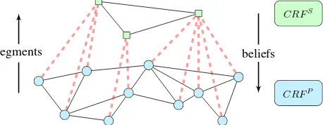
3. HIERARCHICAL CRF
We design a hierarchical CRF consisting of two layers in order to realise the iterative classification of points and segments. The goal is to classify the point cloud as accurately as possible. The CRF layout is shown in Fig. 2. First, we perform a point-based classification on the point layer (CRFP). Subsequently, a sec-ond CRF classification operating on segments is applied. This layer is denoted byCRFS. The segmentation is obtained by detecting connected components of the same class labels in the classified point cloud. Thus, for each segment also a prior of the semantic label is known which can be used for the extraction of features. In this way the result ofCRFP is propagated to CRFS. In contrast, the optimisation ofCRFSdelivers beliefs for each segment to belong to a certain object class. These beliefs are mapped to the point level and incorporated into the next iter-ation of theCRFP via an additional cost term. In this way the results are propagated along the red dashed lines in Fig. 2 from one step to the next. The basic idea and main motivation of this framework is that some remaining classification errors ofCRFP might be eliminated by utilising regional context information be-tween segments instead of points. While local interactions are mainly modelled by the point-basedCRFP, the segment-based CRFSis able to represent longer range interactions at a regional level. The classification in both layers is applied several times in sequence with the aim of improving the segments iteratively, and transferring regional context to the point-based level. The three componentsCRFP, segmentation, andCRFSare described in the following subsections.
segments beliefs
CRFS
CRFP
Figure 2. Hierarchical CRF consisting of a point layer (blue) and a segment layer (green). The black edges model the inter-layer relations. The red dashed lines visualise the intra-layer connec-tions, which are considered by defining the segments on the one hand, and by propagating the beliefs of the segment layer to the point layer on the other hand.
3.1 Point-Based ClassificationCRFP
We start with the description of the point-basedCRFP repre-senting the point layer in our hierarchical framework. Each point represents a node of the graph and is linked by edges to itsk nearest neighbours in 2D. This corresponds to a cylindrical neigh-bourhood which was identified to be more expressive than a spher-ical neighbourhood. In this case also the larger height differences of the points are modelled, which carry helpful information for distinguishing certain classes (Niemeyer et al., 2011). The en-ergy ofCRFPis composed of four terms:
EP(x,y) =X
unaryandpairwise costs, respectively.EP
h(xc)models thehigher
order costfor each cliquec∈C. The parametersθP
p andθhPact as relative weights of the energy components. A second unary termEξP(y
s
i)weighted byθPξ is introduced to incorporate the results of the segment-based classificationySi. The costs are ex-plained in the following subsections.
3.1.1 Unary Cost The unary costEuP(x, yi)determines the most probable object label of them classes for a single node given its feature vectorfP
i(x). For each nodenisuch a vector is extracted taking into account not only the dataxiobserved at that point, but also at the points in a certain neighbourhood. The cost is modelled to be the negative logarithm of the probability of yigiven the datax:
EuP(x, yi) =−logp(yi|f P
i(x)). (3)
Any discriminative classifier with a probabilistic output can be used for the computation of the unary cost (Kumar and Hebert, 2006). In this work, we apply a Random Forest (RF) classifier. (Breiman, 2001). It consists of a number T of trees grown in a training step. In order to classify an unknown sample from the dataset, each tree casts a vote for the most likely class based on its features which are presented to the trees. Dividing the sum of all votes for a class by the total number of trees defines a probability measure which is used in Eq. 3.
3.1.2 Pairwise Cost The termEP
p(x, yi, yj)in Eq. 2
repre-sents the pairwise cost and explicitly incorporates the contextual relations in the classification process. It models the dependencies of a nodenifrom its adjacent nodenjby comparing both node labels and considering the observed datax. We apply a contrast-sensitive Potts model (Boykov et al., 2001), which considers the similarity of both adjacent node feature vectors with its Euclidean distancedij=||fPi(x)−fPj(x)||:
The relative weights of the data-dependent and data-independent smoothing term in Eq. 4 is controlled by the parameterp1 ∈
[0; 1]. Ifp1is set to zero, the degree of smoothing depends com-pletely on the data. In contrast, the model becomes a simple Potts model ifp1 equals one. The parameterσ2
corresponds to the mean value of the squared feature distancesd2ijand is determined during training. The contrast-sensitive Potts model in the point layer classification leads to a data-dependent smoothing effect, preserving small structures with different features.
3.1.3 Higher Order Cost In (Niemeyer et al., 2015) it turned out that many lidar points could not be associated with a segment ofCRFSbecause they were assigned to labels different to their neighbours. Thus, no improvement by the segment-based clas-sification could be obtained for those isolated points. To cope with this problem we additionally make use of the RobustPn Potts model (Kohli et al., 2009) in this study in order to ob-tain a smoother result. Compared to a standard segmentation, the RobustPnPotts model enables a ‘soft‘ segmentation based on higher order cliques. These cliques are provided in advance, i.e. by a segmentation. In order to distinguish between the seg-mentation generating the higher order cliques on the one hand, and the segmentation extracting the entities forCRFS(Section 3.2), we denote the former bySegP n in this paper. The energy termEP
cost. The maximum costγmaxis assigned in case of more thanQ members with a label different than the dominant label. In case of a more homogeneous labelling of the clique members, the cost is linearly reduced depending on the number of variables not taking the dominant label (Kohli et al., 2009):
EhP(xc) =
Our goal is to preserve small structures in the point cloud, on the one hand, and to still obtain smooth results serving as input for the segment layer classificationCRFS, on the other hand. We formulate a cost function depending on the quality and on the size of each clique:
The segment qualityG(x)is defined by the variance of the pos-teriors obtained from the unaries (RF classification, Eq. 3) of all points within one clique. In Eq. 7,µlrepresents the mean value of the probabilities belonging to classl. A high variance indi-cates an inhomogeneous clique, leading to a high cost. In con-trast, a clique with a dominant label provides a low variance. It represents a good homogeneous clique, and thus its nodes should be favoured to be assigned to the same class. θhp1P is a data-independent smoothing term andθP
hp2models the relative weight of the data-dependent term. Both parameters are determined in training. θhp3P is set manually to control the influence on the clique size. The cliques are constructed with the supervoxel-algorithm, which has been shown to provide good segmentation results for point cloud (Papon et al., 2013). Multiple segmenta-tions can be used forSegP n, and the segments are allowed to overlap. In this way segments of different scales can be consid-ered.
3.1.4 Long Range Cost In order to propagate the information obtained by the larger spatial scale of the segment layer to the next iteration ofCRFP, an additional energy termEξP(y
We map the classification results of CRFS to the point level, where each lidar pointiis assigned the beliefs per class of the segment-based classification result. The beliefs are denoted by belS
i(ySi))in Eq. 8. This strategy enables to incorporate the in-formation gained by considering the larger scale into the local point classification.
3.1.5 Features A set of geometrical and waveform based fea-tures is extracted for each 3D lidar point representing the feature vectorfPi(x)for each nodeni. In our casefPi(x)consists of 12 components. The waveform features are theintensity valueas well as theecho ratio, which describes the ratio of the echo num-ber per point and the total numnum-ber of echoes in the waveform. A larger group of features represents the local geometry of the point cloud. These features arelinearity,planarity,scatter,anisotropy,
normal of an approximated plane, and theratio of the sums of the eigenvalues in a 2D and a 3D neighbourhood, which have been shown to lead to good results in (Chehata et al., 2009). The scale of the local neighbourhood for the computation of these features is determined in the way described in Weinmann et al. (2015). Additionally, the featureheight above groundis used. It is ex-tracted using the module LASHeight from the software package
LASTools1. All features of nodes are scaled to the range [0,1].
3.1.6 Training and inference Our framework is a supervised classification method. Thus, we need a fully labelled reference point cloud for the training of the RF classifier as well as of the weightsΘ= (θP
hp1, θPhp2, θPp, θhP).
Learning parameters for higher order random fields is still an active field of research. For our framework we apply a similar heuristic as used by Kohli et al. (2009). Firstly, we learn the rel-ative weightθPp between unary and pairwise potentials without considering higher order cliques. Secondly, the higher order pa-rametersθP
hp1andθPhp2are trained without considering pairwise interactions. The last step is to learn the relative weightingθP h between the pairwise and the higher order interactions. Training of all parameters simultaneously would lead to very low weights for the higher order costs because both interaction potentials have a similar (smoothing) effect on the result (Kohli et al., 2009). We determineΘby maximising the number of correct samples using a part of the training data that was not used for training the en-ergy terms. The relative weightθP
ξ is set manually, but it can be learned based on training data in the future. The contextual term is not yet available in the initial iteration ofCRFP. For this rea-son, the costs are set to be equal for all classes in the first iteration to enable an appropriate training of the relative term weightsθP p andθhP.
Inference is the task of finding the optimal label configuration based on minimizing the energy function of Eq. 2 for given parameters. We use the methodology suggested by Kohli et al. (2009), which is able to perform inference on CRF withPnPotts models very efficiently in low polynominal time with a graph-cut based algorithm (Boykov et al., 2001). In order to integrate the additional energy termEP
ξ(ySi)into this framework, we add the contextual costs to the costs of the unary term for each node.
3.2 Segmentation
Based on the results of the point-based classification, segments are extracted. For this task, Conditional Euclidean Clustering (Rusu, 2009) is applied as implemented in the Point Cloud Li-brary2. It is a variant of a region growing algorithm connecting points which are close to each other and meet additional condi-tions. In our case the points are allowed to have a distancedseg
, and they must have the same label from the point-based classifi-cation to be assigned to the same segment. This leads to a seg-mented point cloud with the advantage of having a prior for the semantic interpretation for each entity, potentially enabling the extraction of more meaningful features for a following segment-based classification.
3.3 Segment-Based ClassificationCRFS
The segments generated in the way described in Section 3.2 are the main entities forCRFSand represent the nodes of the seg-ment layer in our model. Adjacent segseg-ments are linked by edges. The adjacency for constructing the graph is given if individual member points of two segments are neighbours in 2D. This is the case if their distance is smaller than a thresholddSgraph. The idea of using this second layer is the incorporation of a larger spatial scale. This information is integrated via the additional contex-tual energy term in Eq. 2 and is assumed to improve the point-based classification. For this reason the focus ofCRFSis not on
1
http://rapidlasso.com/lastools/ (accessed 07/12/2015) 2
smoothing the labels, but on exploiting context. This CRF utilises only the unary and the pairwise costs with a relative weightθPp:
ES(x,y) =X i∈n
EuS(x, yi) +θSp
X
i,j∈e
EpS(x, yi, yj) (9)
3.3.1 Unary Cost Similar to the point layer, the negative log-arithm of the posterior of a segment-based RF classifier is used to define the unary energyEuS(x, yi).
3.3.2 Pairwise Cost In contrast to the contrast-sensitive Potts model, a generic model of the local relations between the object classes does not only lead to a smoothing effect but is also able to learn that certain class relations may be more likely than oth-ers given the data (Niemeyer et al., 2014). In the segment layer the pairwise costs are modelled by the negative logarithm of the joint posterior probability of two node labelsyiandyjgiven an interaction feature vectorfS
ij(x)for each edgeeij.
EpS(x, yi, yj) =−logp(yi, yj|fSij(x)). (10) This information is used to improve the quality of classification, with the drawback of having to determine more parameters. We apply another RF classifier to obtain the probabilities for the in-teractions in a similar way as for the unary costs. The main differ-ence in this case is thatm2
classes must be distinguished for the pairwise interactions because each object class relation is consid-ered to correspond to a single class.
3.3.3 Features The availability of segments allows for the ex-traction of a new set of features for nodes and their interactions. We extract themean and standard deviation of the point intensi-tiesas well asof the height above the DTM. Moreover, the max-imum difference in elevationis determined. Three features are derived from an approximated plane: thenormal direction, the
standard deviation of the point normal directions, and thesum of the squared residuals. Additionally, three parameters describe the segment geometry: thearea, thevolumeas well as thepoint densitywithin the segment. Themean value of the echo ratio
helps to detect vegetation. Three more features make use of con-text: For each segment themost prominent neighbouring class labelis determined based on the results ofCRFP
by counting the labels of direct neighbour segments and using the label with the maximum vote as a feature.
Inspired by the idea of (Golovinskiy et al., 2009), we use two fea-tures related to roads which are supposed to describe the relative positions of the segments in the scene. For each segment the dis-tance to a roadis computed by searching the closestroadpoints to its centroid. Theorientation with respect to the closest road
is expressed by the angle between the principal direction and the direction from the segment centroid to the closestroadpoint. The principal direction is obtained by a principal component analysis. In total, 15 features compose the segment feature vectorsfSi(x).
InCRFSall potential class relations are distinguished by the in-teraction model. For this reason we have to derive discriminative features for each edge. We use the concatenated node feature vec-tors of both adjacent segments. Additionally, the feature vector is augmented by thedifferences of intensity, height, and normal direction, theminimum Euclidean distancebetween the points of two segments, as well as by themean height differences at the border the segments. This results in an edge feature vectorfS
ij(x) consisting of 35 elements.
3.3.4 Training and inference Two independent RF classifiers have to be trained for the unary and pairwise terms, respectively.
In order to learn the interactions of object classes, a fully labelled reference point cloud is needed. The same training areas are used for both layers. Segments are obtained by classifying the train-ing areas and applytrain-ing the Euclidean clustertrain-ing in the same way as described before. In order to determine the reference labels for these segments, a majority vote of all point labels contribut-ing to one segment is performed. Accordcontribut-ing toCRFP the rela-tive weightθS
p is learned by varying the parameter and selecting the value, which leads to the maximum number of correct sam-ples. For inference the max-sum version of the standard mes-sage passing algorithm Loopy Belief Propagation (LBP) (Frey and MacKay, 1998) is used. Compared to graph-cuts, LBP has the advantage that it does not require the potentials to be submod-ular.
3.4 Alternating optimisation
The two layers of our framework are optimized independently. We do not model the intra-layer edges which are represented by red dashed lines in Fig. 2 explicitly by edges of a CRF. The rea-son for that is that a single inference step solving both layers si-multaneously is difficult to carry out due to the changing graph structure inCRFS. In contrast, information between the layers is propagated in another way with the possibility of enabling an iterative correction of labelling errors. On the one hand, the re-sult of the point-basedCRFP is used to generate the segments serving as input for the segment layerCRFS
. On the other hand, the output of the segment-based classification is propagated into the next iteration ofCRFP via the energy termEξP (Eq. 8). The computations stop after a manually set number of iterations is reached.
Some kind of smoothing is additionally applied by assigning iso-lated points not belonging to any segment (and thus remaining unclassified inCRFS) to the smallest segment in a small spher-ical neighbourhood of radiusriso. In this way they also receive segment beliefs for the next iteration ofCRFP. This may serve as an indicator for the isolated points to be classified in the same way as their neighbouring points. The smallest segment in the neighbourhood is chosen for improving the detection of small structures. For instance, it favours an isolated point with a height of 1 m above the road to belong to the car segment next to it in-stead of being assigned to the significantly largerroadsegment.
With regard to the computational effort note that the point fea-tures used inCRFP have to be extracted only once. On the other hand the contextual costs and the higher order costs change from iteration to iteration and have to be re-computed. It is also possible to re-use the trained RF classifier from the first iteration. ConsideringCRFS, the features have to be extracted in every iteration because the segment borders change. Moreover, both RF classifiers (for the unary and the pairwise terms) are trained anew in each iteration. The global weighting parametersΘare optimised only once during the first iteration.
4. EXPERIMENTS
4.1 Test setup
A training set consisting of 750,440 points is used for learning the RF classifiers. The relative weights of the energy terms are deter-mined using a second training set comprising 411,114 points. The point cloud which is used for evaluation has 1,079,527 points. A manual labelling of all points was performed to obtain reference labels for training and accuracy assessment. We distinguish be-tween the six object classesroad, natural soil, low vegetation,
tree, building, and carin both layers. Note that the different classes do not appear equally often in the data set. In particu-lar,low vegetationandcarare rare.
We use three different settings in order to assess the accuracy of our framework and to determine the benefits of the two suggested road featuresdistanceandorientation to the closest roadfor seg-ments:
1. The first classification uses both road features. For their computation the closest segment which was classified as
road(and is larger than 10 points for robustness) is detected in order to roughly approximate the road. Thus, it is based on the classification results fromCRFP
. This approach is denoted by Rapprox. The parameters are trained using this setting and the results are presented in detail in Section 4.3. 2. In the second classification, denoted as ROSM, an external road data base from OpenStreetMap3is used for the compu-tation of both features. The roads are represented by poly-lines in this case. The aim is to find out if any improvements can be gained compared to using only approximate roads. 3. For evaluating the impact of both road features, a
classifi-cation is performed withoutdistanceandorientation to the closest road. This result is referred to as RnoRoad.
The classification results of ROSM and RnoRoad are compared with Rapproxin Section 4.4.
4.2 Parameters
To ensure a fair comparison, the same parameters were used in all experiments. The trained parameters are obtained from Rapprox. We performed five iterations of the alternating point- and segment-based classification in each case. Moreover, the following param-eters are used:
Point layer: The graph is constructed withk = 7neighbours. p1 of the contrast-sensitive Potts model is set to 0.5 as a trade-off between smoothing and dependence on data. The higher or-der cliques are constructed from the results of two applications of the supervoxel-algorithm (Papon et al., 2013) (SegP n). We use 0.7 m and 1.0 m as different resolutions to obtain segments describing even small objects in a good manner. The number of segmentations as well as their parameters were determined empir-ically. Qis set to30 %,θPξ to 0.5, andθPhp3 to 0.1. The weights
ΘforCRFP
were determined to beθP
hp1 = 0.7,θPhp2 = 5.84, θP
p = 3.55, andθhP = 1.2in training. The RF classifier for the unary potential consists of 200 trees, which are trained based on 5000 samples per class.
Segmentation: Points assigned to the same label are connected if they are closer thandseg
= 1 m. The minimum size for each segment is set to three points to allow for an extraction of repre-sentative segment features (Section 3.3.3).
Segment layer: In training,θSp was determined to be 1.0. The radius for isolated points to be assigned to a segment isriso= 1 m. We use 200 trees with 5000 samples per class for the unary costs, and 200 trees with 3000 samples for the interaction RF due to the lower number of available training samples.
3
www.openstreetmap.org/ (accessed 22/02/2016)
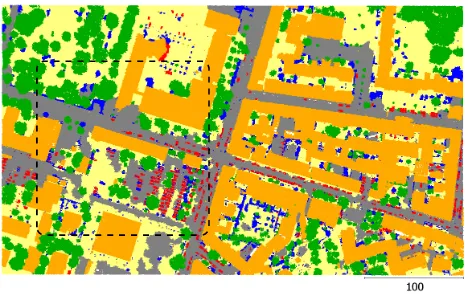
Figure 3. Result of the lastCRFPclassification for the test area. The colors correspond to the classes road(grey), natural soil
(yellow),low vegetation(blue),tree (green),building(orange), and car(red). The dashed rectangle illustrates the location of Fig. 4
.
4.3 Evaluation
The result of our classification scheme for Rapproxis visualised in Fig. 3. The corresponding completeness, correctness as well as quality values per class are presented in Tab. 1 for the final CRFP andCRFSresults. The quality per class is defined as a measure which takes into account the completeness and the cor-rectness (Heipke et al., 1997). The overall accuracy for the test area is 80.4 % for CRFP and 81.1 % forCRFS, which is a reasonable result for the challenging area and the separation of six object classes. The quantitative evaluation in Tab. 1 indi-cates varying accuracies for the different object classes in terms of completeness and correctness.
The best classification results were obtained fortreeandbuilding
with high completeness (>93.5 %) and correctness (>95.9 %) values, resulting in very good quality values. Thus, these two classes are detected reliably in both classifications. By far the most challenging class islow vegetationin this scenario. It has a poor quality of about 19 % (CRFP) and 25 % (CRFS) due to low correctness values. Confusion mainly occurs with the classes
natural soil,building, andtree. Apparently the class oflow veg-etation is not well defined and the features are not expressive enough to distinguish the objects correctly. In particular, objects oflow vegetationshow various appearances in the data. In gen-eral, every class is slightly improved in quality by applying the segment-based classification.
Table 1 additionally provides the difference to the initial point-based classificationCRFP in parenthesis. Positive values (in green) correspond to a better result of our iterative framework. After the first run ofCRFP an overall accuracy of 78.1 % is achieved, which can be used for comparison because no interac-tion with the segment layer took place. This result is improved by alternating through the two layers of our framework. The in-formation mutually propagated between point and segment-based levels increases the overall accuracy by 2.3 % to 80.4 % (CRFP) and by 3.0 % to 81.1 % (CRFS) after five iterations.
Class CRF
P CRFS
Completeness Correctness Quality Completeness Correctness Quality
Road 58.9 (+4.0) 65.7 (+8.2) 45.0 (+6.0) 58.9 (+4.0) 65.7 (+8.2) 45.1 (+6.0) Natural Soil 75.5 (+3.4) 69.9 (+4.5) 56.9 (+4.8) 76.3 (+4.1) 69.8 (+4.4) 57.3 (+5.1) LowVeg 41.7 (+15.1) 26.0 (-1.8) 19.1 (+3.3) 46.1 (+19.4) 34.8 (+7.0) 24.7 (+9.0) Tree 93.5 (+0.1) 95.6 (-1.2) 89.6 (-0.9) 95.1 (+1.6) 95.9 (-0.8) 91.3 (+0.8) Building 95.0 (-0.8) 97.6 (+1.1) 92.8 (+0.3) 95.5 (- 0.3) 97.1 (+0.7) 92.9 (+0.4) Car 52.3 (+34.7) 73.7 (+2.8) 44.1 (+27.6) 47.7 (+30.1) 86.4 (+15.4) 44.4 (+27.9)
Table 1. Completeness, correctness and quality in [%] after the last iteration ofCRFP andCRFS, respectively. The comparison to the first iteration ofCRFP (without any information obtained by segments) is shown in parenthesis. Values in green indicate the improvements of our alternating framework. The overall accuracy is 80.4 % (+2.3) in case ofCRFPand 81.1 % (+3.0) forCRFS.
due to improved completeness values. This can be explained by the fact that some object points were lost due to smoothing in the initial classification because of the RobustPnPotts model. Alsoroad,natural soildandlow vegetationcan be detected more accurately in the point and in the segment layer. These classes benefit from the propagated context information. Some errors in-troduced in the first point-based classification can be corrected in this way. One example is the relatively challenging separation be-tween the classesroadandnatural soilin the data set. The most important feature for their separation is the intensity value of the lidar points. However, there are many macadam roads, parking areas, and pathways (at the cemetery in the upper left part of Fig. 3) which tend to show ambiguous appearance. In some cases our framework is able to correct the initially assigned wrong labels because the shape and the position of the segment are not very likely.
A further advantage of our methodology is the information about segments. In addition to the low level point cloud classification, we obtain segments roughly corresponding to instances of ob-jects, and we also know their class label. This allows us to esti-mate the number of object instances for each class in the scene. For example, we detected 512 car segments in the scene. Figure 4 shows sometreesegments on the left hand side as well as in-dividualcarsegments on the right hand side. Due to the lack of reference data for these objects, we can not perform an qualitative evaluation.
Figure 4. In addition to the point cloud labels, also individual segments approximating the object instances in the scene are de-rived for each class. The left part of this 3D view shows thetree
segments, on the right side individual cars are represented by seg-ments. A greyscale intensity image of the scene is visualised in the background. The location of the scene is illustrated by the dashed rectangle in Fig. 3.
4.4 Road features
This investigation analyses the influence of the two segment fea-turesdistance and orientation to the closest road. The
computa-Class CRF
P CRFS
Rapprox ROSM Rapprox ROSM
Road +3.3 +2.5 +4.0 +3.2
Natural Soil +3.0 +3.3 -1.4 -1.2
Low Veg. -2.5 -0.4 -2.4 -5.0
Tree +1.3 +0.2 +0.9 +0.1
Building +0.6 0.0 +0.1 -1.0
Car -4.7 +2.0 -7.5 +0.8
Overall Accuracy +1.5 +1.3 +0.2 -0.1
Table 2. Comparison of quality values and overall accuracies [%] with respect to RnoRoadto determine the influence of the features
distance to roadandorientation to road.
tion of these features in Rapprox(Section 4.3) was based on an approximation of the road. In this section a comparison to ROSM and RnoRoadas described in Section 4.1 is carried out.
The results are summarised in Tab. 2 by presenting the differ-ences in quality and overall accuracy with respect to RnoRoad af-ter the lastCRFP
andCRFS
classification, respectively. Neg-ative values (in red) indicate a better accuracy of RnoRoad. The features are used at the segment layer and the information is then propagated to the point layer iteration by iteration. It becomes evident that the two introduced road features distanceand ori-entationof segments to roads improve the results for the (final) point layer. The overall accuracies increase by 1.5 % (Rapprox) and 1.3 % (ROSM), respectively. ForCRFSthe impact is only marginal.
Considering the quality values it turns out that 14 of the 24 indi-cators are improved by the new features. In contrast, the quality decreases in 9 cases. In one case no difference was detected. The classroaditself benefits most from the road information. The quality increases by>2.5 %on the point level and by>3.2 % on the segment level.Treeis also affected positively. It becomes apparent that the less prominent classlow vegetationsuffers from the incorporation of these features. Due to the varying shape of low vegetation no representative orientation to the road can be learned. Additionally, the principal direction can not be com-puted robustly for small segments consisting of only a few points. A similar behaviour is observed forcar: the quality is reduced only in case of the approximated road. Apparently, some isolated segments classified asroadon the parking areas distort the fea-tures of some cars in Rapprox. On the other hand, the detection of cars is improved if the OSM data are used, which only contain the skeletons of the roads. Parking areas are not considered in this case, and hence all cars located in this area have more homo-geneous features concerning their orientation and distance to the road polyline.
for the approximated road and the external road database. How-ever, expressive segments are necessary in order to describe the object orientation in an appropriate way. Further investigations will show if these features can be used to improve the detection rate of small classes, too.
5. CONCLUSION AND OUTLOOK
We have proposed a hierarchical classification framework for air-borne lidar point clouds based on a two layer Conditional Ran-dom Field (CRF). Both layers are applied in sequence and in-teract mutually. This approach is able to incorporate local and regional context. In our experiments an increase of 2.3 % (point-based) and 3.0 % (segment-(point-based) in overall accuracy is observed. We could demonstrate that the suggested iterative framework im-proves the classification accuracy and allows for the correction of errors in the previous results at a later stage. In particular, the classcarbenefits from our methodology. Moreover, we in-troduced two new segment features for airborne point clouds de-scribing the distance and the orientation of each segment with re-spect to the closest road. These features are helpful and improve the overall accuracy by up to 1.5 % in our experiments.
In future work we intend to improve the higher order cost func-tionγmaxas well as the road features for a better detection of under-represented object classes. Furthermore, we will evalu-ate the performance of our approach using more test areas with different characteristics, and investigate the required amount of training data.
REFERENCES
Albert, L., Rottensteiner, F. and Heipke, C., 2015. An iterative inference procedure applying Conditional Random Fields for si-multaneous classification of land cover and land use. In: ISPRS Annals of Photogrammetry, Remote Sensing and Spatial Infor-mation Sciences, Vol. II-3/W5, pp. 1–8.
Boykov, Y., Veksler, O. and Zabih, R., 2001. Fast approximate energy minimization via graph cuts. IEEE Transactions on Pat-tern Analysis and Machine Intelligence 23(11), pp. 1222–1239.
Breiman, L., 2001. Random Forests. Machine learning 45(1), pp. 5–32.
Chehata, N., Guo, L. and Mallet, C., 2009. Airborne Lidar Fea-ture Selection for Urban Classification using Random Forests. In: International Archives of Photogrammetry, Remote Sensing and Spatial Information Sciences, Vol. XXXVIIInumber Part3-W8, ISPRS, Paris, France, pp. 207–212.
Frey, B. and MacKay, D. J. C., 1998. A revolution: Belief propa-gation in graphs with cycles. In: Advances in neural information processing systems, Vol. 10, The MIT Press, pp. 479–485.
Golovinskiy, A., Kim, V. G. and Funkhouser, T., 2009. Shape-based recognition of 3D point clouds in urban environments. In: Proceedings of the IEEE International Conference on Computer Vision, pp. 2154–2161.
Gould, S., Rodgers, J., Cohen, D., Elidan, G. and Koller, D., 2008. Multi-class segmentation with relative location prior. In-ternational Journal of Computer Vision 80(3), pp. 300–316.
Heipke, C., Mayer, H., Wiedemann, C. and Jamet, O., 1997. Evaluation of Automatic Road Extraction. In: International Archives of Photogrammetry and Remote Sensing, Vol. 32(3-4W2), pp. 151–156.
Kim, B.-S., Kohli, P. and Savarese, S., 2013. 3D scene under-standing by Voxel-CRF. In: Proceedings of the IEEE Interna-tional Conference on Computer Vision, pp. 1425–1432.
Kohli, P., Ladick´y, L. L. and Torr, P. H. S., 2009. Robust higher order potentials for enforcing label consistency. International Journal of Computer Vision 82(3), pp. 302–324.
Kumar, S. and Hebert, M., 2006. Discriminative Random Fields. International Journal of Computer Vision 68(2), pp. 179–201.
Najafi, M., Namin, S. T., Salzmann, M. and Petersson, L., 2014. Non-associative higher-order markov networks for point cloud classification. In: Proceedings of the European Conference on Computer Vision, Springer, Zurich, pp. 500–515.
Niemeyer, J., Rottensteiner, F. and Soergel, U., 2014. Contextual classification of lidar data and building object detection in urban areas. ISPRS Journal of Photogrammetry and Remote Sensing 87, pp. 152–165.
Niemeyer, J., Rottensteiner, F., Soergel, U. and Heipke, C., 2015. Contextual classification of point clouds using a two-stage CRF. International Archives of the Photogrammetry, Remote Sensing and Spatial Information Sciences XL-3/W2, pp. 141–148.
Niemeyer, J., Wegner, J. D., Mallet, C., Rottensteiner, F. and So-ergel, U., 2011. Conditional Random Fields for urban scene clas-sification with full waveform LiDAR data. In: Photogrammetric Image Analysis, Lecture Notes in Computer Science, Vol. 6952, Springer, Munich, Germany, pp. 233–244.
Papon, J., Abramov, A., Schoeler, M. and Worgotter, F., 2013. Voxel cloud connectivity segmentation - Supervoxels for point clouds. In: Proceedings of the IEEE Conference on Computer Vision and Pattern Recognition, pp. 2027–2034.
Pham, T. T., Reid, I., Latif, Y. and Gould, S., 2015. Hierarchical Higher-order Regression Forest Fields : An application to 3D in-door scene labelling. In: Proceedings of the IEEE International Conference on Computer Vision, pp. 2246–2254.
Rusu, R. B., 2009. Semantic 3D object maps for everyday ma-nipulation in human living environments. PhD thesis, Technische Universit¨at M¨unchen, Germany.
Schindler, K., 2012. An overview and comparison of smooth labeling methods for land-cover classification. IEEE Transactions on Geoscience and Remote Sensing 50(11), pp. 4534–4545.
Sengupta, S. and Sturgess, P., 2015. Semantic Octree : Unifying recognition, reconstruction and representation via an octree con-strained higher order MRF. In: IEEE International Conference on Robotics and Automation, pp. 1874–1879.
Shapovalov, R., Velizhev, A. and Barinova, O., 2010. Non-associative markov networks for 3D point cloud classification. In: International Archives of Photogrammetry, Remote Sensing and Spatial Information Sciences, Vol. 38number 3A, pp. 103–108.
Weinmann, M., Jutzi, B., Hinz, S. and Mallet, C., 2015. Seman-tic point cloud interpretation based on optimal neighborhoods, relevant features and efficient classifiers. ISPRS Journal of Pho-togrammetry and Remote Sensing 105, pp. 286–304.
![Table 1. Completeness, correctness and quality in [%] after the last iteration of CRFimprovements of our alternating framework](https://thumb-ap.123doks.com/thumbv2/123dok/3288825.1403285/7.595.57.291.488.625/table-completeness-correctness-quality-iteration-crfimprovements-alternating-framework.webp)
