Power requirement of swimming in chinook
salmon and Atlantic salmon and implications
for food conversion and growth performance
Royann J. Petrell
a,*, Rachael E. Jones
baDepartment of Chemical and Bio-Resource Engineering,Uni
6ersity of British Columbia,
2357Main Mall,Vancou6er,BC,Canada V6T1Z4
bECL En
6irowest Consultants,Suite204,800McBride Boule6ard,New Westminster, BC,Canada V3L2B8
Received 26 October 1998; accepted 31 January 2000
Abstract
Body dimensions and swimming speeds of Atlantic salmon (Salmo salar) and chinook salmon (Oncorhynchus tshawytscha), ranging in weight from less than 1 to over 6 kg, were used to calculate the power needed to overcome drag. Fish were kept in 15 m×15 m×15 m deep cages, stocked under typical industrial conditions and fed to apparent satiation by broadcasting feed over the water surface. The average swimming speed for both species was 0.68 m s−1. Power required for swimming increased as the fish grew, and at a weight of
1.25 kg, fish changed from using available energy for long distance travelling to carrying a greater amount of weight for a shorter distance. The average profile drag acting on chinook salmon was significantly higher than on Atlantic salmon, principally because the girth of a chinook salmon was significantly larger than the girth of an Atlantic salmon of similar mass. This difference in energy expenditure due to drag explains over 20% of the observed difference in the feed conversion ratios of the two species. The selection of fish with a more streamlined body shape as breeding stock could improve the economics of chinook salmon cultivation. The techniques outlined herein can be used (a) to evaluate suitability of other species and sites for aquaculture, (b) as criteria in a breeding program, and (c) for setting criteria for permissible velocities in fisheries projects. © 2000 Elsevier Science B.V. All rights reserved.
Keywords:Drag; Swimming speed; Feed conversion; Growth
www.elsevier.nl/locate/aqua-online
* Corresponding author. Tel.: +1-604-8222565; fax:+1-604-8225407. E-mail address:[email protected] (R.J. Petrell)
1. Introduction
Under cultivation, farmed chinook salmon have generally higher feed conver-sion ratios (FCRs), higher mortality rates and lower growth rates than Atlantic salmon. The FCR is the ratio of feed fed (kg) to weight gained (kg). Note that throughout this paper, weight (a force with the SI unit of Newton) will have the SI unit of kilogram, normally attributed to mass, following the convention used in fishery science. According to the Cooperative Assessment of Salmonid Health program, which is being conducted through the British Columbia Salmon
Farm-ers’ Association, typical FCR values in British Columbia in 1993 were 1.5 for
Atlantic salmon and 2.0 for chinook salmon over the entire production period. Atlantic salmon also had a much higher average harvest weight, at 4.3 as com-pared with 2.5 kg for chinook salmon over the same growout period (BCMAFF, 1993).
Chinook salmon are considered to be more environmentally sensitive than Atlantic salmon. Chinook salmon show symptoms of oxygen stress when dis-solved oxygen is below saturation, whereas Atlantic salmon tolerate oxygen levels as low as 44% saturation (Caine et al., 1987). Chinook salmon are more sensitive to temperature fluctuations than Atlantic salmon, but Atlantic
salmon become increasingly susceptible to Vibrio infections as salinity levels
drop below 15 parts per thousand (Caine et al., 1987). Atlantic salmon show somewhat faster growth than chinook salmon at temperatures lower than 14°C, which is the optimum temperature for growth for both species (Pennell, 1992). Atlantic salmon can, therefore, be raised where chinook salmon cannot, for example at a site with lower dissolved oxygen levels or greater temperature fluctuations.
Drag increases with swimming speed, bodily area exposed to flow and drag coefficient. Drag has been measured on some fishes (dead drag), but only over a small range of size and shape (e.g. Blake, 1983). Chinook salmon tend to be deeper bodied (with more area exposed to flow) than Atlantic salmon. We hy-pothesized that the higher FCRs and lower growth rates of chinook salmon are due, at least partly, to their higher energy expenditure while swimming. The objectives of this research were to: (1) compare the swimming speeds and body dimensions of the two species over a wide range of size; (2) calculate drag and power; and (3) determine whether differences in FCR and growth rate could be accounted for by differences in body morphology, drag and power.
2. Materials and methods
2.1.Swimming speed data
Average speed, length (taken at the tail fork if present), height (distance between the dorsal and ventral sides at the widest point along a fish) and weight of fish were measured while testing Fish Image Capturing and Sizing System (FICASS) on salmon farms (Shieh, 1996; Jones, 1997). FICASS includes underwater stereo cameras and an image capturing and analysis system (Petrell et al., 1997). To obtain the data, cameras were first lowered into a cage to videotape fish. Images were later used to calculate average swimming speed, length and weight. The number of
images sampled for swimming speed per sampling position,n, within a cage varied
from ten to 60 depending on variability and was calculated for each sampling position using
n=[t2
s2 ]/d2
wheretis the tabulatedtstatistic for a 95% confidence interval,d is the half-width of the confidence interval (for our purposes, it was set to be 0.1 of the average value
of the swimming speed) ands is the sample standard deviation (Steel and Torrie,
1960). The low sample numbers were not considered a statistical concern, as Boisclair (1992) found that sample size did not have a significant influence on mean speed estimates of fish. The same method was used to determine the number of images needed to calculate the average fish weight per sampling position, except that d was set to be 0.05 of the average value of the weight. The sample size varied between 56 and 120 fish. Individual swimming speed and length measurements were
accurate to93%, while measurements on average fish weight were accurate to
97%. Five different farming sites of Atlantic salmon (totaling 26 different cages)
and three farming sites of chinook salmon (totaling 14 different cages) were
sampled to cover the growth cycle for each species ($1 kg to harvest weight). In
total, 24 and 81 measurements of average swimming speed, length and weight were recorded for chinook and Atlantic salmonids, respectively.
Data were taken directly from production cages. Fish were held in cages
15×15×15 m3 deep and were fed by farm workers to apparent satiation by
broadcasting feed over the surface of the cage. Sites were low current sites
(averaging 0.1 m s−1). In addition to fish measurements, water temperature near
the cameras was also measured.
2.2.Body measurements
2.3.Drag and power calculations
Drag arises from two sources, pressure (form) and shear stress (friction drag).
The total or profile drag,D, was calculated using the equation:
D=0.5rCdAV2 (1)
whereVequals swimming speed,r equals fluid density,Cdequals drag coefficient
andAis a reference area. Working estimates of drag coefficient can be determined
from listed data provided shapes are geometrically similar (Gerhart and Gross, 1985). In some previous hydrodynamic models, fish have been assumed to have a streamlined and rotationally symmetrical shape (Blake, 1983; Tang and Wardle, 1992). The drag coefficient we used was calculated as in Eq. (2), assuming a streamlined but not rotationally symmetrical body, similar to an airfoil (Hoerner, 1958).
Cd=2Cf[1+2(H/L)+100(H/L)
4] (2)
For an airfoil,H is the height of the airfoil,Lis the cord length and Cfequals the friction drag coefficient. For our application to be analogous to an airfoil, we have
set H equal to the height of the fish and L equal to the length of the fish. The
friction drag coefficient was calculated using Schoenherr’s formula for turbulent skin friction drag on a plane surface (Hoerner, 1958):
(Cf)−0.5=3.46 log Rl−5.6 (3)
where Rlis the Reynolds number based on fish length (Reynolds number is defined
as velocity times length over kinematic viscosity). In Eq. (2)H/Lis multiplied by two to account for both sides of the fish. Eq. (2) implies that streamlining (elongating the rear portion of the body as reflected in a lowering of theH/Lratio) reduces profile drag. Streamlining for drag reduction is only effective up to a point, as with elongation comes an increase in ‘wetted surface area’ (Eqs. (1) and (3)), which increases friction drag and therefore increases profile drag. Eqs. (2) and (3) were used to calculate the drag coefficient for both chinook salmon and Atlantic salmon because both have the same general shape of an airfoil (see Section 3,
roundness). As well, calculated Rl values indicated that the flow conditions were
turbulent, and theoretical values for the skin friction drag coefficient for a flat plate in turbulent flow have been shown to reasonably approximate the drag coefficient for salmonids (Blake, 1983). Equation 1 calculates the effect of drag quite conserva-tively as actual values would be higher due to turning, fins and added mass (Blake, 1983).
The reference surface area was taken to be the planform area (i.e. the area you would see if you looked at a swimming fish from above (Gerhart and Gross, 1985). Consistent with convention, the platform area of a fish was calculated as its length times its thickness. To obtain a value for thickness, data for girth and height, and the equation representing the perimeter of an ellipse were used as follows. First, the shape of the cross section of a fish at its widest point was assumed to be an ellipse
The perimeter of the ellipse which is defined mathematically to be approximately equal to [2p(0.5(T2+H2))0.5] is therefore equal to the girth of the fish. The
equation for perimeter was then rearranged to solve forT(thickness) given bothH
(height), and perimeter (girth).
To summarize, the drag formula that was used (Eq. (1)) is rewritten below
showing the substitutions forA and Cdto illustrate the reliance that drag has on
differences in body morphology and swimming speed.
D=rTLCf[1+2(H/L)+100(H/L)4]V2
As mentioned previously, drag would increase as the H/L (height/length) ratio increases or the fish becomes more blunt (form drag increases), and/or if the body becomes longer (friction drag increases).
As girth was not measured on all fish, drag was calculated using the average swimming speed found for each species on a subset of the fish (146 individual chinook salmon and 298 Atlantic salmon) ranging in size from 1.0 to 6 kg which had a complete data set of physical measurements of weight, girth, height and length. Power was calculated as drag (Eq. (1)) times swimming speed (Blake, 1983). Both power and drag were graphed against fish weight for both species. To further our understanding of how a fish might use available energy, the power data was also used to calculate the distance a fish could move and the weight a fish could carry given 1 W s of available energy.
2.4.Data transformation and statistical analysis
Regression equations and coefficient of determination (r2
) were calculated to compare relationships between direct measurements of weight and the various dimensions of girth, length and height. For these variables, a power law model (i.e. ln(weight) vs. ln(height)) was tested because the ln transformations were able to produce linear plots. We did not imply by the use of these models a dependence of weight on girth, length or height; rather we used them to compare regression coefficients between species. The average swimming speed of fish at every sampling location in a cage was compiled, and the strength of a relationship between speed,
water temperature and fish weight was determined by calculatingr2. The F
maxtest was used to test homogeneity of variance of swimming speed. Roundness, defined as ‘a measure of the sharpness of the corners of a solid’, was also examined (Mohsenin, 1986). Roundness of a fish was calculated as girth (or circumference)/
P/height (or diameter). The strength of the straight-line relationship between
roundness and fish weight was determined by calculating r2
.
For comparison of regression parameters between species, a modifiedt-test was
used. The t-test was used for comparison of means between species (i.e. for
roundness, speed). Normality was verified using Kolmogorov-Smirnov goodness of fit tests, and homogeneity of variance was tested with the Hartley test.
2.5.Effect of swimming on growth
To examine the effect of swimming on growth, the total daily energy require-ments for fish were compared to the energy requirerequire-ments for swimming and growth only. Values for the total energy required were obtained from literature while the energy required for swimming was calculated using our calculated values of power, as follows.
The total daily energy requirement was found by analyzing feed components, and assuming satiation and a balanced diet. Commercial salmon feeds are high-energy
diets comprised of44% protein and 23% oil (Jackson, 1988). The average caloric
value of these two major energy sources, corrected for digestibility and the portion present as nitrogen (and therefore unavailable as energy) is 3.9 kcal g−1
of protein and 8.0 kcal g−1
of fat (Phillips, 1972). Based on these values and the percent breakdown of the diet, 1 kg of food has a total of 3556 kcal of energy from protein and oil. This translates into a total of 16.0 kcal (kg fish)−1day−1(calculated with
a ration level of 4.5×10⁻³ kg of feed (kg fish)−1 day−1, which is the
recom-mended level for salmonids weighing over 2 kg in 8°C water (Moore Clark Feed Tables, 1993)).
The total energy requirements of swimming (W s) as a fraction of the energy available in the diet can be calculated by integration (i.e. determining the area under the curve generated by plotting power required for swimming against time). However, our data produced plots of power against fish weight. To perform the integration, the unit of mass (horizontal axis) was converted to time by calculating the time needed to grow from one size class to another. Hence, a 1 kg-sized fish might represent 100 days and a 2 kg-sized fish, 200 days. The transformation from weight to time was achieved by employing the standard exponential growth
equation and published growth rates,m (day−1) as below:
Time (days)=(lnWt2−lnWt1)m
−1
where Wt2 and Wt1 represent fish weights at the end and beginning of a growth
period, respectively. For this analysis the class size change during a growth period was set at 0.5 kg. The average growth rates of Atlantic salmon at 8 – 12°C and ranging in size from 150 to 3000 g were obtained from Austreng et al. (1987). They
range from 1.9 to 0.67% day−1. The growth rates of chinook salmon were set in a
lower range to reflect the fact that they grow to a size of 2.5 kg during the same time period it takes to produce a 4.3 kg Atlantic salmon.
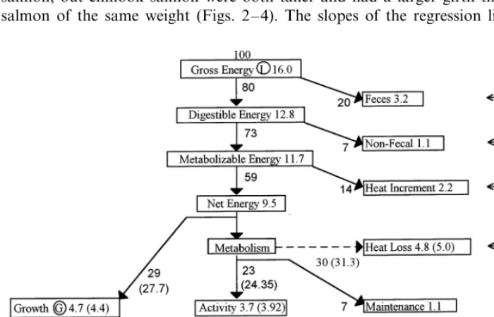
Next, the percentages of the energy budget used for swimming and growth were determined. Published mass-balance equations provided the means of modeling the partitioning of food energy between the various metabolic processes within a fish, such as tissue function and repair, synthesis of new tissue, and swimming. An
energy budget for an individual fish takes the basic form:I=M+G+EwhereIis
the energy content of the food consumed over the time period,Mis the energy lost
in the form of heat produced during metabolism,G is the energy in both somatic
and reproductive growth, andEis the energy lost in faecal and excretory products
balanced energy budget of a carnivorous fish (based on published data for 15 species of fish); 100I=(4497)M+(2996)G+(2793)E(Brett and Groves, 1979).
The total metabolism can be further broken down into standard metabolism (MS),
feeding metabolism (MF), active metabolism (MA) including swimming, and the
heat increment, or energy of specific dynamic action (SDA) (Fig. 1). The above numeric model was used to reflect the change in growth due to a change in energy expenditure due to swimming. For example, if a species used 10% instead of 6.75% of its available energy for swimming, then according to Fig. 1 the energy available for growth would decrease from 29% of total energy to 25.75%.
3. Results
3.1.Shape
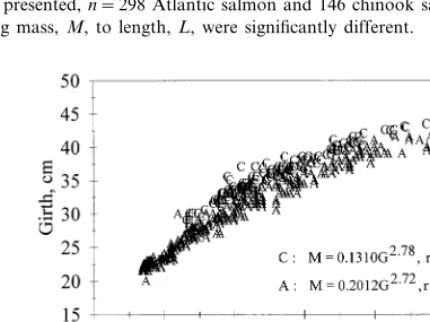
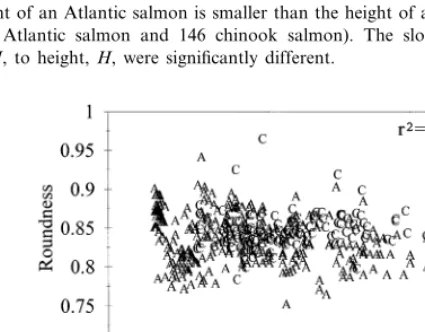
When both species were examined together, some interesting trends became evident. For fish of the same mass, Atlantic salmon were longer than chinook salmon, but chinook salmon were both taller and had a larger girth than Atlantic salmon of the same weight (Figs. 2 – 4). The slopes of the regression lines for the
Fig. 1. The energy budget of 3 kg-sized Atlantic and chinook salmon. The values within the boxes are in units of kcal (kg fish−1) day−1; values beside the arrows are percentages. The circled lettering
Fig. 2. Atlantic salmon are longer than chinook salmon of the same weight (for clarity, only a subset of available data is presented,n=298 Atlantic salmon and 146 chinook salmon). Slopes in the regression equations relating mass,M, to length,L, were significantly different.
Fig. 3. The girth of an Atlantic salmon is smaller than the girth of a chinook salmon of comparable weight (n=298 Atlantic salmon and 146 chinook salmon). The y constants in the regression equations relating mass,M, to girth,G, were significantly different.
transformed variables of length and weight, and height and weight for the two species were significantly different (differences of they-intercepts were not tested),
but was not significantly different for girth and weight. The y-intercepts for the
regression lines for girth and weight were, however, significantly different.
fishes tended to have elliptically shaped cross sections (height\thickness). Round-ness did not correlate to fish weight. It can be ascertained from these results (roundness, height and girth) that the thickness of a chinook salmon is greater than the thickness of an Atlantic salmon of similar weight.
Fig. 4. The height of an Atlantic salmon is smaller than the height of a chinook salmon of comparable weight (n=298 Atlantic salmon and 146 chinook salmon). The slopes in the regression equations relating mass,M, to height,H, were significantly different.
Fig. 6. The average swimming speed of farmed salmon was 0.68 m s−1. Each point represents the
average speed found at a camera position in a cage. The standard deviation at each position for chinook salmon was 930 – 40% of the value, while it was only97% for Atlantic salmon. All data came from low current velocity salmon farming sites.
3.2.Swimming speed
As a general observation, the variation in swimming speed at any camera
position was significantly higher for chinook (930 – 40% of the average positional
speed) than for Altantic salmon (97% of the average positional speed). From the
video footage, chinook salmon exhibited far more darting, acceleration and direc-tional changes than Atlantic salmon; in other words, they seemed ‘wilder’ and responded much more readily to outside stimuli, while the Atlantic salmon behaved in a more domesticated fashion. Swimming for all positions and species was quasi-steady; fish coasted between bouts of acceleration.
After averaging together all the positional swimming speeds, the overall average swimming speeds for both species were 0.68 m s−1(not significantly different). The swimming speed obtained at each camera position did not correlate with the mean positional fish weight (Fig. 6), water temperature or time of day (for details on temperature and time of day, see Jones, 1997). Water temperature varied depending on the time of year between 7 and 14°C.
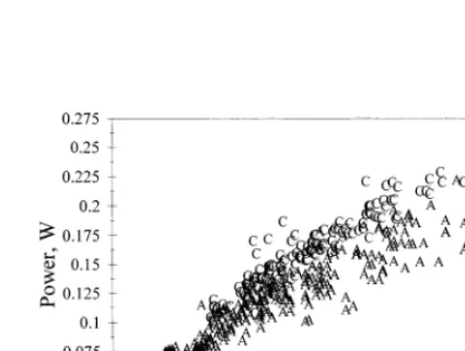
3.3.Drag and power
Both drag and power (Fig. 7) increased as individual fish weight increased. For Atlantic salmon, power requirements tended to level off after a fish reached 3.5 kg in size. A visual comparison of the curves for each species showed that the power
requirement of a 2 – 4 kg chinook salmon was 20% higher than the power
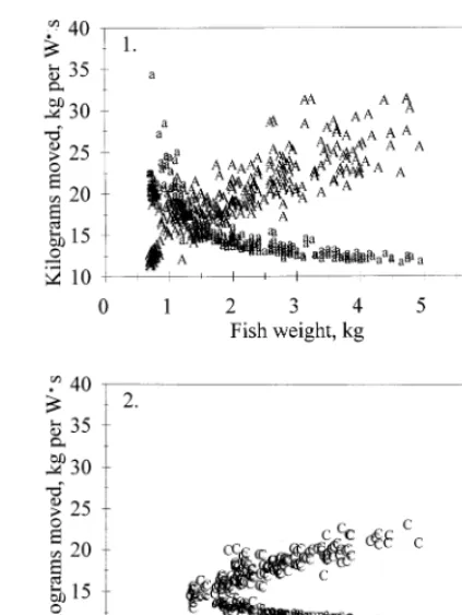
When comparing how the two species use available energy, some interesting trends became evident (Fig. 8). The curve representing the distance different sizes of fish could move on 1 W s of energy was hyperbolic. This trend is more easily seen for Atlantic salmon, as a wider range of data were available for Atlantic salmon than chinook salmon. The inflection point on the curve occurred between 1 and 1.5 kg of weight. Fish smaller than 1 – 1.5 kg moved a much greater distance per 1 W s of available energy than larger fish.
The curve representing how much weight a fish could move per 1 W s of available energy was also non-linear (Fig. 8). For both species, as fish increased in weight they became more efficient carriers of weight. The chinook salmon was always less efficient as it could carry less weight given the same amount of available energy than an Atlantic salmon of similar size. An inflection point occurred in the curve at an approximate weight of 1.25 kg for Atlantic salmon (as before, insufficient data were available for chinook salmon). Therefore, after 1.25 kg, fish changed from being efficient long distance travelers to efficient carriers of weight (Fig. 8).
3.4.Effect on growth
The energy requirement due to swimming varied as the fish grew, increasing from 2% of the total energy supplied for a 1 kg fish to 6.7% for a 3 kg Atlantic salmon (Figure not shown, as the shape is similar to Fig. 7). The energy requirement due to swimming for a chinook salmon was 20% higher throughout the same time interval. This increased cost of swimming for chinook salmon decreases the amount
of energy available for growth by 4.5% day−1
(4.5=100(29−27.7)/29 see Fig. 1).
Fig. 8. Utilization of available energy for swimming: (1) Atlantic salmon; (2) chinook salmon. For Atlantic salmon the shape of the two curves had an inflection point at1.25 kg. Prior to that size, fish could travel further on a unit of energy, while after that size, fish could carry more weight per unit of energy.
4. Discussion
This research is the first where fish speed is measured and drag is calculated over a wide range of fish sizes under field conditions. Average swimming speed (0.68 m s−1) was within the range of values found by other researchers on salmonid species (e.g. Malinin, 1975; Beamish, 1978; Bell, 1986), but significantly lower than the criterion (2.7 m s−1) for designing safe salmonid passage at sustained speeds (Dane, 1978). Fish forced to swim at the tabulated sustained speeds would have an energy requirement for swimming 57 times higher than the energy required to swim at 0.7
m s−1, as power requirements increase with the cube of velocity.
twice, both before and after meals. Boucher and Petrell found that time of day affected swimming speed in 13 out of 18 cages of salmon, and although the difference in swimming speed among cages was not tested, their data indicates the variation in swimming speed between cages was probably as high as the temporal effect.
The power needed to overcome the drag force ranged between 0.05 and 0.25 W. These values are similar to experimental values found for Atlantic salmon and other salmonids (Blake, 1983; Tang and Wardle, 1992). Webb (1991) supports elevating drag based on average swimming speed by a factor of three to account for quasi-steady swimming. This would increase the percentage of gross energy spent on swimming for each species by a factor of three in our study. Differences between species would, however, remain the same.
Chinook salmon had a higher energy cost for swimming than Atlantic salmon (by 20% over the same production period). To compensate for this, the growth rate of chinook salmon would be lower than Atlantic salmon at the same ration level. This difference in growth explains 20% of the 33% difference between typical FCR values of 1.5 for Atlantic salmon and 2.0 for chinook salmon in 1993. The sudden darts and directional changes by swimming chinook salmon may be another cause of the consistently poorer performance of chinook salmon as compared to Atlantic salmon. By observation, chinook salmon exhibited a swimming behaviour that could be characterized as routine swimming, while Atlantic salmon tended to demonstrate a directed swimming pattern (as defined by Boisclair and Tang, 1993). The aforementioned researchers found that routine swimming was 4.9 – 7.5 times more expensive than directed swimming for fish of similar weight. Taking the difference in the form of swimming into account (by multiplying the power
requirements of swimming for chinook salmon by 5) would explain 75% of the
difference between the FCR values of the two species.
The increasing usage of available energy for swimming in chinook salmon as compared to Atlantic salmon explains why chinook salmon cannot attain the same harvest weight as Atlantic salmon (4.5 kg) during the same time period or with the same ration. The swimming behaviour of wild salmon in the ocean has not been well documented. Perhaps chinook salmon, the least streamlined of the two fishes studied, tends to swim with the current rather than against it, or shelter behind objects such as rock outcroppings to escape the strongest currents.
As the average swimming speed of the two species was nearly identical, the difference in drag on the two species is due to body form. To lower the FCR for chinook salmon, a more streamlined fish can be selected and cultivated.
Finally, both species undergo a change at 1.25 kg, which effects how the fish
Our procedures involving the measurement of swimming speed and fish, and the use of equations which took into consideration the body shape, provide a way for farmers to assess and compare the power requirements of swimming. These methods could be applied to identifying suitable low energy consuming alternative aquaculture species provided data on swimming speed, overall energy usage and morphology is available. They can, in addition, be used to develop a breeding program and set limits on current. Where chinook and Atlantic salmonids must swim against the current, it is reasonable to say velocities should not exceed 0.3 m s−1. In this way fish would make reasonable forward motion at 0.68 m s−1without exceeding normal swimming power requirements.
Acknowledgements
Appreciation is extended to the National Science and Engineering Research Council of Canada and to the four fish farming companies (B.C. Packers, Pacific Salmon Farming Partners, Pacific National and Paradise Bay Seafarms) for their support.
References
Austreng, E., Storebakken, T., A8sga¨rd, T., 1987. Growth rate estimates for cultured Atlantic salmon and rainbow trout. Aquaculture 60, 157 – 160.
BC Ministry of Agriculture, Fisheries and Food (BCMAFF), 1993. Aquaculture: Its Role in British Columbia’s Seafood Industry. British Columbia Ministry of Agriculture, Fisheries and Food, Victoria, BC, p. 7.
Beamish, F.W.H., 1978. Swimming capacity. In: Hoar, W.S., Randall, D.J., Brett, J.R. (Eds.), Fish Physiology. Locomotion, vol. VII. Academic Press, London, pp. 101 – 187.
Bell, M.C., 1986. Fisheries Handbook of Engineering Requirements and Biological Criteria. US Department of Commerce, Springfield, VA, pp. 282.
Blake, R.W., 1983. Fish Location. Cambridge University Press, New York, p. 208.
Boisclair, D., 1992. An evaluation of the stereocinematographic method to estimate fish swimming speed. Can. J. Fish. Aquat. Sci. 49, 523 – 531.
Boisclair, D., Tang, M., 1993. Empirical analysis of the influence of swimming pattern on the energetic cost of swimming in fishes. J. Fish Biol. 42, 169 – 183.
Boucher, E., Petrell, R.J., 1999. Swimming speed and morphological features of mixed populations of early maturing and non-maturing fish. Aquacul. Eng. 20, 21 – 35.
Brett, J.R., Groves, T.D.D., 1979. Physiological energetics. In: Hoar, W.S., Randall, D.J., Brett, J.R. (Eds.), Fish Physiology. Bioenergetics and Growth, vol. VIII. Academic Press, London, pp. 279 – 352. Caine, G., Truscott, J., Reid, S., Ricker, K., 1987. Biophysical Criteria for Siting Salmon Farms in British Columbia. B.C. Ministry of Agriculture and Fisheries, Aquaculture and Commercial Fish-eries Branch, Victoria, BC and Aquaculture Association of British Columbia, p. 50.
Dane, B.G., 1978. A review and resolution of fish passage problems at culvert sites in British Columbia, 4th edn. Department of Fisheries and Environment, Pacific Region, Fisheries and Marine Service Technical Report no. 810, p. 120.
Gerhart, P.M., Gross, R.J., 1985. Fundamentals of Fluid Mechanics. Addison-Wesley, Reading, MA, pp. 509 – 539.
Jackson, A., 1988. Growth, nutrition and feeding. In: Laird, L.M., Needham, T. Jr (Eds.), Salmon and Trout Farming. Ellis Horwood, Chichester, pp. 202 – 216.
Jones, R.E., 1997. Comparison of some physical characteristics of salmonids under culture conditions using underwater video imaging techniques. MSc Thesis, University of British Columbia, Vancouver, p. 107.
Malinin, L.K., 1975. Rates of movement of salmon (Salmo salar) during anadromous migration in fresh water. Zoologicheskii Shurnal LIV, 1729 – 1731.
Mohsenin, N., 1986. Physical Properties of Plant and Animal Materials. Gordon and Breach Science Publishers, New York, p. 84.
Pennell, W., 1992. Site Selection Handbook. BC Ministry of Agriculture, Fisheries and Food, Victoria, BC.
Petrell, R.J., Shi, X., Ward, R.K., Naiberg, A., Savage, C.R., 1997. Determining fish size and swimming speed in cages and tanks using video techniques. Aquacul. Eng. 16 (1,2), 63 – 84.
Phillips, A.M. Jr, 1972. Calorie and energy requirement. In: Halver, J.E. (Ed.), Fish Nutrition. Academic Press, New York, pp. 2 – 27.
Shieh, A., 1996. Fish size estimation in sea cages using a fish image capturing and sizing system. MSc Thesis, University of British Columbia, Vancouver, p. 120.
Steel, G.D., Torrie, J.H., 1960. Principles and Procedures of Statistics. McGraw-Hill, New York, pp. 86 – 87.
Tang, J., Wardle, C.S., 1992. Power output of two sizes of Atlantic salmon (Salmo Salar) at their maximum sustained swimming speeds. J. Exp. Biol. 166, 33 – 46.
Webb, P.W., 1991. Composition and mechanics of routine swimming of rainbow trout,Oncorhynchus mykiss. Can. J. Fish. Aquat. Sci. 48, 583 – 590.
Wootton, R.J., 1990. Ecology of Teleost Fishes. Chapman and Hall, New York, p. 404.