HEAT TRANSFER TO FLUIDS IN LAMINAR FLOW THROUGH DUCTS
MOHD KHAIRI BIN ABDULLAH
This PSM is submitted to Faculty of Mechanical Engineering Universiti Teknikal Malaysia Melaka in partial fulfillment for Bachelor of Mechanical Engineering
(Thermal Fluid)
Faculty of Mechanical Engineering
Universiti Teknikal Malaysia Melaka
‘Saya/Kami* akui bahawa telah membaca karya ini dan pada pandangan saya/kami* karya ini
adalah memadai dari segi skop dan kualiti untuk tujuan penganugerahan Ijazah Sarjana Muda Kejuruteraan Mekanikal (Termal-Bendalir)’
Tandatangan μ……….. Nama Penyelia Iμ……….. Tarikh μ……….
i
ACKNOWLEDGEMENT
Alhamdulillah with his Mercy and Blessings, my greatest attitude to Allah the Almighty for the chances given to me to complete this project. My first acknowledgement goes to Mr. Shamsul Bahari bin Azraai, my project supervisor. Thanks for his tremendous help, advice, inspiration and unending guidance to me until completing this thesis. Without him, this project will not exist. The fundamental idea behind this project is his and he never stop from giving me support and encouragement in completing this project. Without his valuable guidance, I would not have been able to achieve the objectivity of this project.
Not forgotten to my beloved parents, Mr. Abdullah bin Hj. Mohamad and Mrs. Saudah bt Jusoh. Your love and caring really touch me. Thanks so much for giving me lifelong encouragement, inspiration and support. May Allah bless both of you.
ABSTRACT
iii
ABSTRAK
CONTENTS
LIST OF ABBREVIATIONS ix
CHAPTER 1.0 INTRODUCTION
1.1 Introduction 1
1.2 Objectives 2
1.3 Scopes 2
1.4 Problem Statement 2 CHAPTER 2.0 LITERATURE REVIEW
LIST OF FIGURES 2.2 Laminar and turbulent velocity profiles 6 2.3 Geometry and coordinate system of square duct 7 2.4 (a)Rectangular duct
(b) Circular duct
7 8 2.5 Laminar heat transfer in square duct flow 8 2.6 (a)Nusselt number vs Graetz number of 4000 wppm with
different Reynolds number
(b) Nusselt number vs Graetz number of 8000 wppm with different Reynolds number
10
10
2.7 Comparison calculated Nusselt numbers for H1 boundary condition
12
2.8 Effect of mesh refinement 12
2.9 Geometry of helical square duct 13
3.1 CFX Flow Chart 15
The Velocity Profile of air inlet velocity 5m/s The Velocity Profile of air inlet velocity 10m/s The Pressure Profiles of air inlet velocity 5m/s The Pressure Profiles of air inlet velocity 10m/s
vii
4.5 4.6 4.7 4.8 4.9 4.10
The Velocity Profile of air inlet velocity 5 m/s The Velocity Profile of air inlet velocity 10m/s The Pressure Profiles of air inlet velocity 5m/s The Pressure Profiles of air inlet velocity 10m/s Comparison Table of Air Through the Duct CFD and Analytical Data versus Duct Location
LIST OF SYMBOLS
Vs = Mean fluid velocity, [ 1
ms ] L = Characteristic length, [ 2
m ] μ = Dynamic fluid viscosity, [ 2
Nsm ]
D = Hydraulic diameter [m]
ix
LIST OF ABBREVIATIONS
CFD = Computational fluids dynamics
CHAPTER 1.0
INTRODUCTION
1.1 Introduction
The study of the fluid flow through different duct geometry is important of its wide use. This is also because with different duct geometry the heat transfer rate also changes. The thermal boundary conditions that need to be considered were also complex and the temperature possibilities are also different. A clear understanding of the thermal boundary condition is important in order to understand the heat transfer problem.
2
1.2 Objective
The main objective of the study is to study the velocity and pressure profile.
1.3 Scopes
The scopes of the study are stated below;
To study the fluid flow through duct To design the duct geometry
To simulate fluid flow through duct using CFD
1.4 Problem Statement
They are several shapes that are being investigated. The shapes of the duct to be investigated are square and circular.
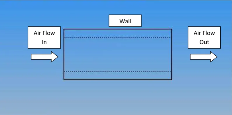
Figure 1.1: Air flow through duct
Air flows through a duct at specified temperature and at different velocity ranging from 5m/s – 10m/s. Ansys CFX is used to stimulated fluid flow through a duct. Finally the results will show the velocity and pressure profile.
Air Flow In
CHAPTER 2.0
LITERITURE REVIEW
2.1 Heat Transfer
Heat transfer is the passage of thermal energy from a hot to a cold body. When an object or fluid is at a different temperature than its surroundings, the transfer of thermal energy also known as heat transfer, occurs that the body and the surroundings reach thermal equilibrium. From the second law of thermodynamics, heat transfer always occurs from a hot body to a cold one. Heat transfer can never be stopped. It can only be slowed down.
2.2 Laminar Flow
Laminar flow also known as streamline flow occurs when a fluid flows in parallel layers, with no disruption between the layers. In fluid dynamics, laminar flow is a flow characterized by high momentum diffusion, low momentum convection, pressure and velocity independent from time. Laminar flow is also called “smooth” in nonscientific terms.
The Reynolds number is an important parameter in the equations that describe whether flow conditions lead to laminar or turbulent flow. In laminar flow,
4
much greater than inertial forces, occurs when the Reynolds number is much less than 1.
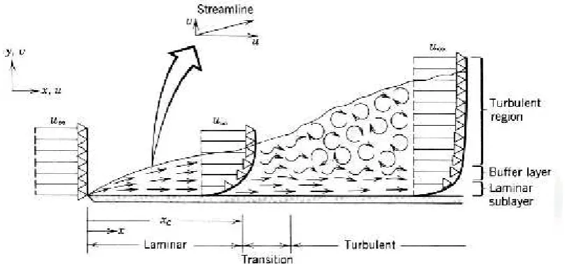
If the flow is laminar, water enters into the water block and flows through the block in nice even layers. Molecules of water stay in the same layer of water as they continue on their path. The molecules of water closest to the water block will be the hottest and moving the slowest, and those in the center of the flow will be the coolest and moving the fastest. This holds true for the entire path through the block and out the exit. The Figure 2.1 shows the boundary layer when the air flow through a flat plate. The first portion is laminar flow.
Figure 2.1: Air flow through a flat plate.
2.3 Reynolds Number
The Reynolds number is the ratio of inertial forces to viscous forces (μ/L) and consequently it quantifies the relative importance of these two types of forces for given flow conditions. Thus, it is used to identify different flow regimes, such as laminar or turbulent flow.
determining dynamic similitude. When two geometrically similar flow patterns, in different fluids with possibly different flow rates, have the same values for the relevant dimensionless numbers, they are said to be dynamically similar. It is named after Osborne Reynolds (1842–1912), who proposed it in 1883.
The Reynolds number can be defining as;
Re
v L v
s/
Laminar flow is smooth and occurs at low Reynolds numbers, where viscous forces are dominant, constant fluid motion, while turbulent flow, on the other hand, occurs at high Reynolds numbers and is dominated by inertial forces, producing random flow, and other flow fluctuations.
The Reynolds number for laminar flow on flat plate is under
2.4 Computational Fluid Dynamics
6
2.5 Boundary Layer
When an object moves through a fluid, the molecules of the fluid near the object are disturbed and move around the object [6]. Aerodynamic forces are generated between the fluid and the object. The magnitude of these forces depends on the shape of the object, the speed of the object and the mass of the fluid. The Figure 2.2 shows the laminar and turbulent velocity profiles.
Figure 2.2: Laminar and turbulent velocity profiles
When a fluid moves past a surface, some of it will stick to the surface (usually the molecules that near the surface). So the other fluid molecules above it will slow down due to the collision between each other. This happens to all layer of the fluid until the layer that is far from the surface. The farther the molecules from the surface less collision or none will happen. This creates a thin layer of fluid near the surface in which the velocity changes from zero at the surface to the free stream value away from the surface. The thin layer is the boundary layer.
2.6 Laminar flow through duct
were higher, up to 300% than the value for the purely forced convection by a Newtonian fluid. The study of the heat transfer and flow characteristics in rectangular duct has become important because of its high heat transfer enhancement than the circular duct or tube [2]. The Figure 2.3 shows the geometry and coordinate system of square duct.
Figure 2.3: Geometry and coordinate system of square duct
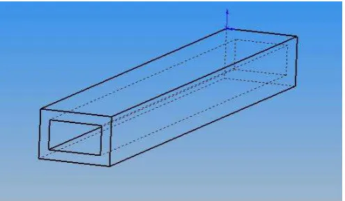
There is several type of duct. The Figure 2.4 shows the isometric drawing of rectangular duct (a) and circular duct (b).
8
Figure 2.4(b): Circular duct
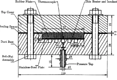
Figure 2.5: Laminar heat transfer in square duct flow
conductivity of about 0.14 W 1 1
m k . To ensure the accuracy of measurements, five
uniformly placed square ducts of the same hydraulic diameter (
D
h = 0.4 cm) wereused. The top wall is a 0.9 mm thick stainless steel plate, and is heated from outside by a 0.08 mm thick electro thermal band under constant heat flux boundary conditions. The entrance to the square ducts is sharp, so the simultaneously developing flows can be generated. The ratio of the duct length to hydraulic
diameter, L D
/
dis 600, thus fully developed flow and heat transfer results can beobtained. The mixing section following the test section is used to provide an equalized bulk fluid temperature. After recovering the heat gain of the test fluid by a heat exchanger, the experimental set-up lets the fluid either go to the weighing tank for mass flow rate measurement or return to the bottom tank for recirculation.
As only the top wall is heated, the buoyancy effects on the non-Newtonian fluid flow through the ducts should be very weak. An analysis has shown that the effects of the heat conduction from the duct walls are also very small within the investigated parameter ranges.
In this experiment the test fluids were use is non-Newtonian aqueous carboxymethyllcelulose (CMC) solutions which are viscoelastic. The aqueous CMC solutions with concentrations of 4000 and 8000 wppm were used in the experiment. In order to clearly define the test fluids, the apparent viscosities of the fluids were measured before and after each heat transfer run. By measured in the rotational viscometer the apparent viscosity of the 8000 wppm aqueous CMC solution is higher than that of the 4000 wppm aqueous CMC solution.
10
In the figure below shows the Nusselt number versus Graetz number (Nux vs Graetz) for the 4000 and 8000 wppm aqueous CMC solutions. The graph also shown for reference is the fully developed Nusselt number (forced convection limit) [3] calculated for a Newtonian fluid in a square duct with only one of the duct wall heated with H1 boundary condition(thermal boundary condition representing constant wall heat flux axially and constant temperature peripherally on one wall of the square duct)
The Figure 2.6 (a) and (b) shows the Nusselt number vs Graetz number of 4000 and 8000 wppm with different Reynolds number.
Figure 2.6 (a): Nusselt number vs Graetz number of 4000 wppm with different Reynolds number
Figure 2.6 (b): Nusselt number vs Graetz number of 8000 wppm with different Reynolds number
flow through a non-circular duct. For a higher concentration, higher heat transfer also increase with aqueous CMC solution and can be produced at higher Reynolds number [3]. As we can see for 4000 concentration, the Reynolds number must be higher enough to enhance the higher heat transfer. While for the 8000 concentration, the heat transfer can be increased at the low Reynolds number.
As we can see in the figures, the 8000 aqueous CMC solution on the laminar heat transfer in square duct is much stronger than the 4000 aqueous CMC solution. At the nearly same Reynolds number we can see that;
4000
2.714exp(0.00349
)
We can conclude here the heat transfer rate also depends on the concentration of the fluid that we use. The high concentration of the fluid must be use to get higher heat transfer.
In the other experiment by Parviz [4], is to explore the suitability of various constitutive models for the prediction of heat transfer to laminar flow of viscoelastic fluids through ducts of noncircular cross-section. The objective of the study is to explore the suitability of constitutive equations which take into account nonzero normal stress coefficients for laminar heat transfer prediction of viscoelastic fluids. In the equation that were made the normal stress coefficient is negligible in longitudinal pressure gradient. This is also because the higher range of Reynolds number was use in the study.
The heat transfer terms that was use;
12
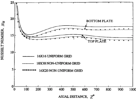
The Figure 2.7 shows the comparison calculated Nusselt numbers for H1 boundary condition. The thermal boundary conditions were used for the top and bottom walls are H1 (at these walls the average heat flux is independent of axial location, while at a given axial location each wall is at a peripherally uniform temperature). The other two side walls are insulated. The Figure 2.8 shows the effect of mesh refinement that was use in the previous study of Parviz [4].
Figure 2.7: Comparison calculated Nusselt numbers for H1 boundary condition
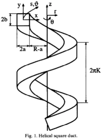
In the study of C.Jonas Bolinder [5], for laminar flow the increased heat transfer is more in the curved duct than the straight duct. For turbulent flow the curved had no other advantages than space saving. The Figure 2.9 shows the geometry of helical square duct.
Figure 2.9: Geometry of helical square duct
In this helical square duct, the wall area is larger than a straight duct since the material had been stretch non-uniformly to obtain the cross section. So there will be more heat transport.
2.7 Continuity Equation