Dynamic Mathematical Modeling and Simulation Study of Small
Scale Autonomous Hovercraft
M. Z. A. Rashid
1, M. S. M. Aras
1, M. A. Kassim
1, Z. Ibrahim
1and A. Jamali
21
Faculty of Electrical Engineering,
Universiti Teknikal Malaysia Melaka, Hang Tuah Jaya, 76100 Durian Tunggal, Melaka, Malaysia
2
Faculty of Mechanical And Manufacturing Engineering,
Universiti Malaysia Sarawak, 94300 Kota Samarahan, Sarawak, Malaysia [email protected]
Abstract
Nowadays, various mechanical, electrical systems or combination of both systems are used tohelp or ease human beings either during the daily life activity or during the worst condition faced by them. The system that can be used to increase human life quality are such as in military operations, pipeline survey, agricultural operations and border patrol. The worst condition that normally faced by human are such as earthquake, flood, nuclear reactors explosion and etc. One of the combinations of both systems is unmanned hovercraft system which is still not thoroughly explored and designed. Hovercraft is a machine that can move on the land surface or water and it is supported by cushion that has high compressed air inside. The cushion is a close canvas and better known as a skirt. A hovercraft moves on most of surfaces either in rough, soft or slippery condition will be developed. The main idea for this project is to develop a dynamic modelling and controller for autonomous hovercraft. The model of the hovercraft will be initially calculated using Euler Lagrange method. The model of the hovercraft is derived using Maple software. The model that is developed then needs to be tested with open loop simulation in the MATLAB/Simulink environment. The LQR controller to regulate the small scale autonomous hovercraft then will be developed and tested with MATLAB.
Keywords: Autonomous, Hovercraft, Dynamic Modelling, LQR regulator
1. Introduction
of damage on its skirt or cushion. There are various type of hovercrafts projects that have been constructed from small scale science projects to racing quality hovercrafts.
2. Literature Survey
The previous studies conducted by several researchers focused on a few types of hovercraft ranging from the human driven hovercraft till the remotely control hovercraft.
In the paper done by [1], the vehicle used LCAC-1 Navy Assault Hovercraft as his case study. This vehicle was designed to be used to transport U.S Marine fighting forces from naval ships off-shore to inland combat position. The journal dismissed a few type of information such as how the driver regulated the surge, sway and the angular velocities of this vehicle. Two different control strategies had been adopted to stabilize the surge, sway and angular velocities with different controllers. The author used the surge force and the angular torque as inputs to the system. In addition, the mathematical model was derived based on
Newton’s Second Law and Euler Lagrange Formulation. The controller that was used in the
journal was based on Lyapunov controller.
Next, the paper done by [2] focused on the hovercraft model namely as Caltech Multi-Vehicle Wireless Testbed (MVVT). This vehicle was equipped by two high powered ducted fans where each fans can produce up to 4.5N of continuous thrust for forward motion. The software that was used in the experiment for position tracking control of an under actuated hovercraft is RHexLib. It was a module-based controller design environment where each module was given an initially fixed execution rate and a module manager performed a static scheduling of the set of modules. The software used by author consists of Lab Positioning System (LPS), Vision Module and Device Writer. The core MVWT modules were Vision Module, which processed broadcasts from the LPS while the controller executed the local
control to determine the vehicle’s position, orientation and identity. In addition, the Device
Writer was used to send the signals to command the fan forces.
The paper [2] considered the position tracking control problem of an under-actuated hovercraft vehicle and used a nonlinear Lyapunov based control algorithm to obtain global stability and exponential convergence of the position tracking error. They mentioned two types of experiments have been conducted to ensure the hovercraft followed a circular desired trajectory.
The hovercraft used by [3] consists of four propulsion motors and they were mounted parallel to the ground in each translational direction to ensure the hovercraft capable to move in any direction. A microcontroller acquired inputs data from the sensors and provided outputs signals to vary the speed of each motor and then perform the necessary stabilization.
In the design, proportional integral derivative (PID) controller was selected to control the hovercraft.
In the book written by [4], the author used Electro Cruiser, an amphibious hovercraft as his experimental model. An electric motor was used to drive both propellers and another one of the propeller to provide lift by keeping a low pressure air cavity inside the skirt. In order to analyze the hovercraft model, the author derived a dynamical model of the hovercraft with the Newton-Euler method. The author only conducted the simulation study and not tested the controller strategy with the real hardware.
speed is the main factor caused the change of hydrodynamic and aerodynamic coefficient of hovercraft. [5] used PID controllers to control the multiple models of the hovercraft. The experiments results showed that MMA had better control effect with a smaller steady state error even though the hovercraft speed was varied.
In [6], the authors studied a toy CD hovercraft to prove the lubrication theory described by the Stokes equation. The theories explored by using this toy CD hovercraft are such as measurements of the air flow value, the pressure in the balloon and of the thickness of the air film under the hovercraft which allowed them to evaluate the Reynolds number R*. Furthermore, they also explored the lifting force applied on the toy of hovercraft and calculated the pressure gradient in the air flow. They also mentioned that the results can be used at a larger scale hovercraft.
In the reference [7], a simple triple hovercraft platform was equipped with fuzzy controller to control the hovercraft. The authors mentioned that the difficulties to control hovercraft arouse like the ability to maintain both manoeuvrability and controllability in any surface especially when the hovercraft starts to move. In the hovercraft development, they used a triangular Stryrofoam as the hovercraft’s frame, three model size airplane motors, three light weight model size airplane propellers, two sensors and interfacing cables. The three motors mounted in a triangular configuration on the Stryrofoam platform. They chose Styrofoam because this material is quite light enough to provide sufficient lift. They also mentioned that the advantage of using fuzzy logic control is the computer can make changes and implement any possible situations within micro-seconds.
In the journal [8], a remote controlled hovercraft had two thrust fans and these lift fan provided two separate sources of input. The author developed mathematical model of the
hovercraft using Newton’s Second Law where the hovercraft had two thrust fans and another
one for lift fan. In addition, the hovercraft had two wires equally spaced from the center of the gravity. The model then transferred into Simulink for simulation to test open loop and closed loop behaviour of the system. The author mentioned that the mathematical model was successfully and accurately controlled.
3. Dynamic Modeling of the System
The small scale autonomous hovercraft in this paper is derived by using Euler Lagrange method. The Euler Lagrange differential equation is derived from the fundamental equation of calculus variations. It states that:
(1)
where:
(2)
(3)
and q is differentiable, and while is derivative of q,
(4)
where:
Lx and Ly denote the partial derivatives of L with respect to the second and third arguments, respectively.
In order to obtain equations of motion for a system with the Euler Lagrange, kinetic energy T, and the potential energy V need to be considered to get Langrangian L= T - V.
The Euler Lagrange equation is shown in Equation (5):
(5)
.
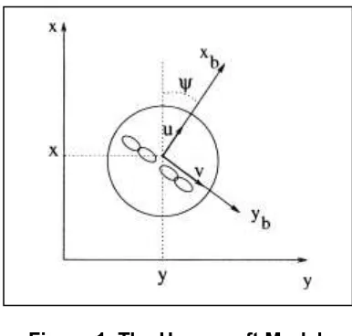
Furthermore, by using Equation (5), the hovercraft model can be further elaborated based on the Figure 1.
Figure 1. The Hovercraft Model
From the Figure 1, the motion equation that involved the hovercraft can be expressed in the Equation (6) to Equation (8):
(6)
(7)
(8)
where:
u is surge velocity v is sway velocity r is yaw angular velocity
The Lagrangian function is shown is Equation (9) and further elaborated in Equation (10) to Equation (12).
(9)
(10)
(11)
(12)
where KE is kinetic energy which is the combination of translational kinetic energy (KT) and rotational kinetic energy (KR). PE in the Equation (12) is the Potential Energy for the hovercraft model. However, in this derivation, Potential Energy for system lifting is neglected and only focuses on the direction movement only. The reason for this assumption is to simplify the derivation.
(13)
The equation of motion then further derived using Euler-Lagrange equation that includes the forces to control the motion.
(16)
where:
,
τ is torque input for the system.
Based on Equation (16), Equation (17) – Equation (25) can be generated.
(17)
(18)
(19)
(20)
(21)
(22)
(14)
(23)
(24)
(25)
where:
is acceleration in surge
.
is acceleration in sway.
is angular acceleration in yaw.
Equation (17) – Equation (25) then can be rearranged and shown in Equation
(26).
(26)
where:
n is number of velocities parameters use where u,v,and r.
r is number of input torque where when input torque are τu and τr. M(q) is a symmetric positive definite inertia matrix with dimension
is centripetal and coriolismatrix with dimension
G(q) is the gravitational terms.
is bounded unknown disturbances including unstructured unmodeled dynamics E(q) is the input transformation matrix with
is the input vector with
is associated with the constraints and its dimension given by
is vector of constraint forces
By using the Equation (26) , the Equation (27) can be obtained.
(27)
where:
Property for M(q) should be symmetric and positive definite where the determinant (M(q)) should be not equal to 0.
From the matrix M(q), the determinant is equal to:
.
By using weight of hovercraft is, m = 2.1kg and angle of rotation . From the parameters of m and angle, the matrix M(q) = 4.41 is larger than 0, then it is proved M(q) is positive definite.
(28)
(29)
In order to test for symmetric,
M(q)–
M(q)T = 0.(30)
Hence, from the Equation (30), it is proven that the
M (q)is symmetric.
The Equation (26) then reorganized to depict the non-linear equation for the system’s investigated and shown in Equation (31).
(31)
(32)
(33)
where f(x) has 2n x1 matrix while B(x) has 2n x 1 matrix.
(34)
(35)
where:
and
(36)
The Equation (31) can be shown as Equation (38) as below,
(38)
(39)
(40)
where:
and the torque to be applied and control the system is shown in the Equation (41).
(41)
where:
τ
uis torque in surge while
τ
ris torque in yaw.
Before the controller for the system is designed, the system needs to be linearized and linearized model is shown in the Equation (42).
(42)
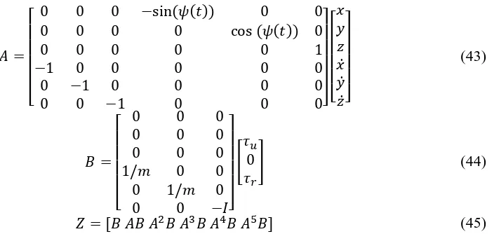
(43)
(44)
(45)
The system controllability is shown in the Equation (45) where if det(Z) > 0, this linearized system is controllable.
The parameters that are used in the equation are:
mass, m =2.1kg
angle, t
and moment of inertia, I=0.000257kgm2
The states are tested either controllable or not by using a matlab command as the following:
p = 30
A = [0 0 0 -sin(p) 0 0 ; 0 0 0 0 cos(p) 0 ; 0 0 0 0 0 1 ; -1 0 0 0 0 0 ; 0 -1 0 0 0 0 ; 0 0 -1 0 0 0]
B = [0 0 0 ; 0 0 0 ; 0 0 0 ; 1/2.1 0 0; 0 1/2.1 0 ; 0 0 -0.000257] Co=ctrb(A,B)
unco = length(A)-rank(Co)
If the result for the system shown unco = 0, the equation system is controllable. In this equation, this command has produced the following result:
unco =0 and the result shows that the equation is controllable.
4. System Controller
The system need to be controlled by certain controller so that it can follow certain trajectories. In this paper, Linear Quadratic Regulation (LQR) is chosen as the controller. Linear Quadratic Regulation (LQR) is a controller that provides control performance with respect to some initial setting condition. State space model is a model that relates input and output of a system using first order-vector differential equation as the following.
where A is n x n matrix, B is a n x m matrix, C is a k x n matrix and D is k x m matrix.
The matrix A and B are inserted into the state space block model in the Simulink / Matlab environment as shown in the Figure 2.
It is assumed that the system have full state feedback by finding the vector K, where the feedback control law is determined. The placed command could be used to determine feedback is the desired closed loop poles are known. In addition, LQR also can be used using the LQR function with two parameters R and Q are chosen which will balance the relative importance of the input and state.
The LQR method allows for control of many outputs where in this project are to control six outputs. The controller can be tuned by changing nonzero elements in the Q matrix to get desirable response. The Q matrix needs to identify before the K matrix is determined to produce a good controller by running the m-file code in Matlab. From the coding in the M-file with the changes in the Q matrix and K matrix, the response can be plotted so that changes can be made in the control and it can be automatically seen in the system output.
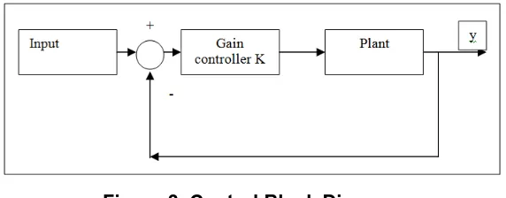
In addition, by using the method mentioned previouspy, a LQR controller design with the position x, position y, position z, and velocities are considered. The equation inside the state space has been determined from the mathematical modelling using Euler Lagrange Method and the equation is linearized to get first order-vector differential equation. This problem can be solved using full state feedback and the schematic diagram of control system can be shown in Figure 3.
Figure 3. Control Block Diagram
There six states
represent the positions and velocities of the hovercraft where LQR controller will be designed with three step inputs. After the linearization of mathematical model is done, the equation is tested in open loop to prove that the system is unstable in open loop.
After the open loop is tested, the next step is to assume that the system have full state feedback by finding the vector gain K to determine the feedback control law. In the feedback controller for the closed loop test, all the feedback states will multiply with the chosen gain K matrix. By running the coding in m-file, the step response simulation is plotted to compare with output open loop and to meet the requirements for the system. The LQR controller can control a multi output system and control the linearized model.
4.1 Open Loop Test
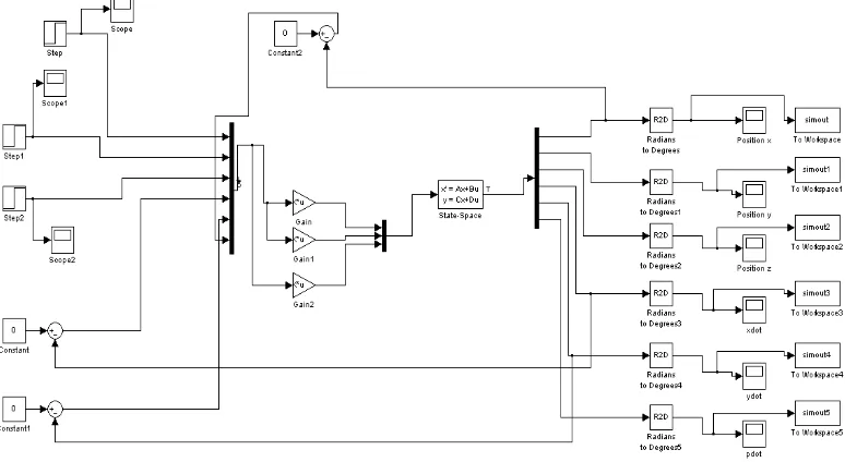
The Figure 4 shows the model in Simulink environment to test the hovercraft system.
There are three sine waves input on the left of the model where τu, τv and τr as input for the
hovercraft system. n the right of this lock shows that outputs for the system where there
are si ouputs, ,y, , ,y , ]^T. When the simulation is run, the input sine will give signal to
Figure 4. Open Loop Diagram for Hovercraft Model Developed
4.2 Close Loop Test
The matrix gain K is used to place the poles of the closed loop system in the open left hand plane of the system using the Matlab command. The system was placed into the block diagram form shown in Figure 5. The state space block holds the adjusted linear model in the matrix form. The linear model was used as a first step in the process to control the nonlinear hovercraft model.
5. Results
5.1 Open Loop Test
A simple coding in m-file will define the state-space function to ensure the open loop test can be run and simulation is plotted. The coding such as the following:
A = [0 0 0 -sin(30) 0 0 ; 0 0 0 0 cos(30) 0 ; 0 0 0 0 0 1 ; -1 0 0 0 0 0 ; 0 -1 0 0 0 0 ; 0 0 -1 0 0 0]
B = [0 0 0 ; 0 0 0 ; 0 0 0 ; 1/2.1 0 0; 0 1/2.1 0 ; 0 0 -0.000257]
C = eye(6)
D = eye(6,3)
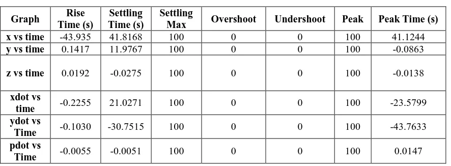
The Table 1 shows the information from simulation open loop test by utilizing the parameters that previously determined.
Table 1. Result for Open Loop Test
Graph Rise
Time (s)
Settling Time (s)
Settling
Max Overshoot Undershoot Peak Peak Time (s)
x vs time -43.935 41.8168 100 0 0 100 41.1244
y vs time 0.1417 11.9767 100 0 0 100 -0.0863
z vs time 0.0192 -0.0275 100 0 0 100 -0.0138
xdot vs
time -0.2255 21.0271 100 0 0 100 -23.5799
ydot vs
Time -0.1030 -30.7515 100 0 0 100 -43.7633
pdot vs
Time -0.0055 -0.0051 100 0 0 100 0.0147
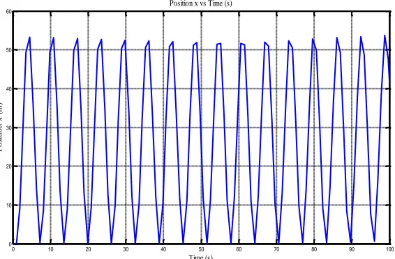
From the table 1, the results for open loop test of the model developed then are further depicted using the graphs.
Figure 6. Surge Position x (m) versus Time (s)
In another figure, Figure 7 shows the position in sway, y (m) vs time (s), where the model start at position 17m in sway at time,t= 0s. Then the model changes its position between -17m to 17m continuously when the time increases. It shows that, the open loop test for the system is not stable in sway position because the hovercraft tends to move from left to right continuously and hardly maintains its position. The hovercraft model cannot be used if the position always changes. It shows that, the open loop are not stable in sway position because the hovercraft move from left to right continuously without maintaining its position. The hovercraft model cannot be use if the position always changes.
Figure 7. Sway Position, y (m) versus Time (s)
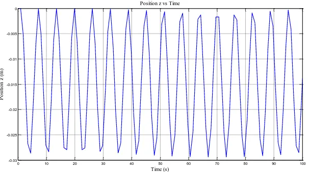
Next, Figure 8 elucidates the yaw position (m) versus time (s). From the graph yaw position in the Figure 8, the hovercraft model always rotate and it is not stable in yaw position. The position is from zero to -0.03m in position z and it continuously. The hovercraft model has little move only position z and because it focus the movement in surge or forward.
0 10 20 30 40 50 60 70 80 90 100
0 10 20 30 40 50 60
Time (s)
P
o
si
ti
o
n
x
(
m
)
Position x vs Time (s)
0 10 20 30 40 50 60 70 80 90 100
-20 -15 -10 -5 0 5 10 15 20
Time (s)
P
o
si
ti
o
n
y
(
m
)
Figure 8. Graph yaw Position (m) versus Time (s)
In the open loop test in order to find the behavior of the velocities of hovercraft model, the velocities graphs are plotted. Figure 9 shows the velocities of the hovercraft in surge (m/s) versus time (s) oscillates continuously from 30m/s to -30m/s. The velocity of the open loop hovercraft model is not stable because there is no feedback from the controller to maintain and to control the velocities of the model. The velocities always increase and decrease causing difficulty controlling forward or surge speed hovercraft
.
Figure 9. Surge Velocity (m/s) versus Time (s)
In the Figure 10, the graph shows the response in the velocities sway versus time is sinusoidal and the range of the velocities is from 40m/s to -40m/s. It is continuous response and it shows the hovercraft movement is not stable because the velocities always increase and decrease. The open loop test is fail to control the velocity of hovercraft.
0 10 20 30 40 50 60 70 80 90 100
-0.03 -0.025 -0.02 -0.015 -0.01 -0.005 0
Time (s)
P
o
si
ti
o
n
z
(
m
)
Position z vs Time
0 10 20 30 40 50 60 70 80 90 100
-30 -20 -10 0 10 20 30
Time (s)
V
el
o
ci
ti
es
u
(
m
/s
)
Figure 10. Sway Velocity (m/s ) versus Time (s)
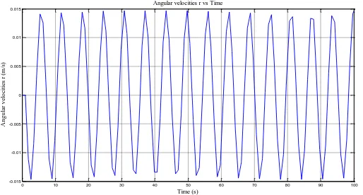
Figure 11 shows the angular velocity of yaw versus time (s) and the graph continuously oscillates in the range from -0.015 m/s until 0.015 m/s. Based on the graph in the Figure 11, the hovercraft model does not spin very quickly even though the time difference is small and this is happen when the angular velocities near to zero.
Figure 11. Angular Velocity, yaw (m/s) versus Time (s)
5.2 Close Loop Test
The system controller gain K can be determined by initially setting matrix Q and matrix R. The matrix value for Q can be set as:
Matrix Q:
8 0 0 0 0 0
0 6 0 0 0 0
0 0 4 0 0 0
0 0 0 2 0 0
0 0 0 0 0 0
0 0 0 0 0 0
0 10 20 30 40 50 60 70 80 90 100
-50 -40 -30 -20 -10 0 10 20 30 40 50 Time (s) V el o ci ti es v ( m /s )
Velocities v vs Time
0 10 20 30 40 50 60 70 80 90 100
-0.015 -0.01 -0.005 0 0.005 0.01 0.015 Time (s) A n g u la r v el o ci ti es r ( m /s )
Matrix R:
0.1 0 0
0 0.1 0
0 0 0.1
By using the state space A and B founded previously, gain values K can be stated as: k1 = [7.0875 -0.0000 0.0000 7.0293 -0.0000 -0.0000]
k2 = [0.0000 5.9256 0.0000 -0.0000 1.9593 0.0000] k3 = [0.0000 -0.0000 -0.0051 0.0000 -0.0000 -6.3246]
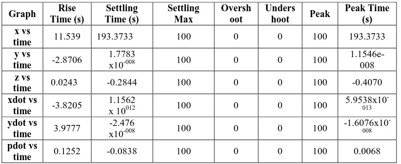
From the gain values K, the gain values then are inserted into the Simulink block diagram. The information from the simulation run are summarized in the table 2:
Table 2. Result Summary for the Close Loop Test
Graph Rise
Time (s) Settling Time (s) Settling Max Oversh oot Unders
hoot Peak
Peak Time (s) x vs
time 11.539 193.3733 100 0 0 100 193.3733
y vs
time -2.8706
1.7783
x10-008 100 0 0 100
1.1546e-008
z vs
time 0.0243 -0.2844 100 0 0 100 -0.4070
xdot vs
time -3.8205
1.1562
x 10012 100 0 0 100
5.9538x10
-013
ydot vs
time 3.9777
-2.476
x10-008 100 0 0 100
-1.6076x10
-008
pdot vs
time 0.1252 -0.0838 100 0 0 100 0.0068
From the Table 2, the performance of the controller is further elaborated through the graph plotted. Figure 12 shows the position of the hovercraft versus time is plotted.
Figure 12. Surge Position x (m) vs Time (s) under LQR Controller
From the graph in the Figure 12, the graph increases from 0m and maintain its position to 193m when the time reaches t= 20s. The rise time for the graph is 11.54s. From this graph,
0 10 20 30 40 50 60 70 80 90 100
0 20 40 60 80 100 120 140 160 180 200 Time (s) P o si ti o n x (m )
the surge position of hovercraft model has improved for the closed loop test using the LQR controller. By using this controller, it can be seen that the hovercraft can be stabilized in surge or when the hovercraft moves forward. The error happen in open loop can be reduced by using the LQR controller especially when the model moves forward.
In another figure, Figure 13 elucidates the graph of y position (m) versus time, t(s) is plotted.
Figure 13. Sway Position y (m) versus Time (s) under LQR Controller
In the Figure 13 above, the graph decreases from 17m to zero position within time t=20s after the simulation of the hovercraft model is started. The rise time of the graph is in negative which is t=2.87s. This show that the hovercraft model position is reduced to become more stable in sway position. The motion of the hovercraft in sway is more stable when it is under controller compared to motion of the hovercraft without using LQR controller.
Figure 14. Yaw Position z (m) versus Time (s) under LQR Controller
From the graph in Figure 14, the position of the hovercraft decreases with time and at time, t= 20s, the position is considered has stabilized and maintained its position. If the black line in the graph represent as the average value of the graph, then the value is -0.33m and it is fix in yaw position which is almost equal to zero position of the hovercraft model. The LQR controller has improved the yaw position in closed loop test although it still has vibration similarly as the yaw position in open loop test.
0 10 20 30 40 50 60 70 80 90 100
0 2 4 6 8 10 12 14 16 18
Time(s)
P
o
st
io
n
y
(m
)
Position y(m) vs Time(s)
0 10 20 30 40 50 60 70 80 90 100
-0.45 -0.4 -0.35 -0.3 -0.25 -0.2 -0.15 -0.1 -0.05 0 0.05
Time (s)
P
o
si
ti
o
n
z
(
m
)
In the next three figures, the surge velocity, sway velocity and yaw velocity will be clearly shown. In the Figure 15, the surge velocity versus time is plotted.
Figure 15. Surge Velocity (m/s) versus Time (s) under LQR Controller
The velocity in surge initially increases then goes down to reach and maintain at zero m/s. This behavior shows that the system is stable when the system is under controller and the controller can control the surge velocity. The velocity in surge is steady in the zero after time,t=20s. The LQR controller helps to stabilize the velocities in surge to ensure the hovercraft moves forward with certain surge velocities and no disturbance occur.
Figure 16. Sway Velocity (m/s) versus Time (s) under LQR Controller
Figure 16 shows the plotted graph of the sway velocity versus time for the model under the LQR controller. From the graph in Figure 16 above, the velocity for sway is equal to zero after time reaches t= 20s although it is initially decreased at the beginning of the graph. This behavior is due to the physical origin where two competing effects which are the fast dynamics and slow dynamic effects, collaborating to generate a negative response prior to starting recover the steps to resolve the steady state positive value based on (Wilkie et al, 2005). Therefore, to avoid this, then a gain [-1] shall be placed on model output.
0 10 20 30 40 50 60 70 80 90 100
0 5 10 15 20 25 30 35 40 45 50
Time (s)
V
el
o
ci
ti
es
u
(
m
/s
)
Graf velocities u vs Time
0 10 20 30 40 50 60 70 80 90 100
-16 -14 -12 -10 -8 -6 -4 -2 0 2
Time (s)
V
el
o
ci
ti
es
v
(
m
/s
)
Figure 17. Yaw Velocity (m/s) versus Time (s) under LQR Controller
The yaw velocity of the hovercraft model is depicted in Figure 17. From the graph , the angular velocity has a wide range from 0.1m/s to -0.1m/s until the final running time, t=100s Even though the velocity in yaw oscillates, it is still better than the graph for angular velocities in open loop test. From the graph, it can be said that that yaw rotation is slow based on the angular velocity in yaw. This indicates that the model of the hovercraft does not experienced spinning movement from the original position.
6. Conclusion
After the completion the project, the linearized mathematical model is successfully derived by using the Euler Lagrange method and suitable control method has been found to control the unmanned hovercraft. From the earlier discussion in the previous subtopic, it can be concluded the Linear Quadratic Regulator (LQR) is suitable controller method to control the hovercraft model for multi inputs and multi outputs of the model. Then, the model is tested in the Simulink/MATLAB software and the graphs are plotted to see the hovercraft model can be stabilized or not. Every controller responses are plotted and then summarized in table. It is found that the LQR is suitable to control the model compared to the open loop where the open loop cannot do the stabilization process. Although the LQR controller has successfully stabilized the system model, implementation of the mathematical algorithm into the real hardware is quite important since the this system is still under simulation study. Therefore implementation into real system will give great advantages to test the algorithm used in the project. The controller technique also needs to be improved in order to obtain a better robust controller and possess better response.
7. Acknowledgement
The authors want express appreciation to Universiti Teknikal Malaysia Melaka (UTeM) for sponsoring this project.
References
[1] I. Fantoni, “ Non-Linear control for Underactuated Mechanical System”, Springer-Verlag London, (2002). [2] A. P. Aguiar, L. Cremean and J. P. Hespanha, “Position Tracking for a Nonlinear Underactuated
Hovercraft:Controller Design and Experimental Results”, California Institute of Technology: Department of Mechanical Engineering, (2003).
[3] A. L. Marconett, “A Study and Implementation of an Autonomous Control System for a Vehicle in the Zero Drag Environment of Space”, University Of California Davis, (2003).
0 10 20 30 40 50 60 70 80 90 100
-0.15 -0.1 -0.05 0 0.05 0.1
Time (s)
A
n
g
u
la
r
v
el
o
ci
ti
es
r
[4] R. M. W. Sanders, “Control od a Model Sized Hovercraft”, The University of New South Wales Australia.
(2003).
[5] W. Cheng-long, L. Zhen-ye, F. Ming-yu and B. Xin-qian, “Amphibious Hovercraft Course Control Based Adaptive Multiple Model Approach”, presented at International Conference on Mechatronics and Automation, (2010).
[6] D. I. Charles and D. I. Gregoire, “Stokes Equation in a Toy CD Hovercraft”, University d’ rleans France,
(2010).
[7] T. Eddie, H. Steve and J. Mo, “Fuzzy Control of a Hovercraft Platform”, Elsevier Science Ltd Printed in Great Britain, (1994).
[8] H. Lindsey, “Hovercraft Kinematic Modelling”, Center of Applied Mathematics University of St. Thomas,