One of the key issue that needs to be addressed in the wireless sensor network field is how to create a most efficient energy system. This is a crucial element because the wireless sensor network is a network made up of small batteries powered devices with a limited amount of energy resources within it. The purpose of the routing protocol is how to utilize energy efficiently and to prolong network lifetime. The conventional clustering method has a unique potential to be an important element for energy conserving sensor network. To address this problem in this paper, we present A Cluster Based Energy Efficient Location Routing Protocol (CELRP) in Wireless Sensor Networks. This routing adopted hierarchical structure method, multi hop and location*based node in the field area of the sensor node. The processes of the routing involves the clustering of nodes and the selection of a Cluster Head (CH) node in each cluster which will be the messenger that sends all the information to the Cluster Head Leader. This Cluster Head Leader will then finally send the aggregated data to the Base Station (BS). To prove the efficiency of energy in CELRP network, we have compared it to the BCDCP and GPRS in the simulation conducted. BCDCP and GPRS are both routing protocols that work well in a small*scale network however not so much in a larger scale network since it uses a lot of energy for long distance wireless communication. The Simulation results have proved energy efficiency in CELRP, its’ ability to reduce energy dissipation and prolong network lifetime that is superior compared to the BCDCP and GPRS.
Wireless Sensor Networks, Clustering, Routing Protocol, BCDCP, GPRS, CELRP.
I. INTRODUCTION
ANY new routing protocols are proposed for Wireless Sensor Networks (WSNs). Recent advances in wireless communication and electronics have enabled the development of low cost, low power, small sized sensor node. In WSNs sensor nodes can be deployed to collect useful information from the field. The energy efficiency is the most important factor, to prolong network lifetime and balance energy consumption. Routing is an important issue that affects wireless sensor networks [4], [24]. One of the energy efficient routing protocols is the Base Station Controlled Dynamic Clustering Protocol (BCDCP) [11] which improves LEACH [14]*[15] from two Manuscript received March 22, 2011.This work was supported in part by the BK 21, Republic of Korea
Nurhayati, Sung Hee Choi and Kyung Oh Lee are with the Computer Science and Engineering Department, Sun Moon University, Kalsanri * Tangjeongmyeon, Chungnam, Asan*si 336*708 Korea (corresponding author to provide phone:+82–41*5302211; e*mail: [email protected], {shchoi, leeko}@sunmoon.ac.kr).
aspects. Firstly, BCDCP uses Minimal Spanning Tree (MST) [5] to connect CHs and randomly chooses a leader to send data to the Base Station (BS). Secondly, BCDCP makes the best use of high*energy BS to choose CHs and form clusters by iterative cluster splitting algorithm. BCDCP reduces far more energy dissipation of network than LEACH but their network topology constraints them from being applicable in large scale network. Geographic routing uses the physical location as the node address [6], [12]. The source node determines the destination address by looking it up from the location server [7], or by computing it using a hash function in a data*centric storage scheme [13]. The node usually forwards the packet to a neighbor closer to the destination. This, however, may take the packet to a dead*end node, that is, a node with no neighbor closer to the destination. In GPSR [1], the algorithm is used on a planar graph to deal with the dead*end node problem.
Position based routing protocols exploit positional information to direct flooding towards the destination in order to reduce overheads and power consumption, Location Aided Routing Protocol (LAR) [21], GRID [18],
Compass [3], and Greedy Perimeter Stateless Routing (GPSR) [2] are examples of position based routing protocols.
The limited energy resources of the deployed sensor nodes are one of the most restrictive factors on the lifetime of wireless sensor networks. In order to achieve high energy efficiency and assure long network lifetime, sensor nodes can be organized hierarchically by grouping them into clusters, where data is collected and processed locally at the cluster head nodes before being sent to a base station. In many sensor network applications where data collection and processing can be done in place, this hierarchical approach is a promising method for efficiently organizing the network.
The main goal of routing protocol in wireless sensor network is to find a way to improve energy efficiency for reliable transmission of sent data to the base station. Almost all the routing protocols can be classified according to the network structure as flat, hierarchical and location*based [9]. Normally, a classical hierarchical routing tactics are of two kinds; distributed routing and centralized routing.
Routing technique of clustering objects is of two types: single*hop and multi*hop communication. In single*hop communication, every sensor node can directly reach the destination, while in multi*hop communication, nodes have limited transmission range and therefore are forced to route their data over several hops until the data reach the final
A Cluster Based Energy Efficient Location
Routing Protocol in Wireless Sensor Networks
Nurhayati, Sung Hee Choi, and Kyung Oh Lee
destination. In both models, there is an unavoidable problem of unbalanced energy dissipation among different nodes, leading to the situation where some nodes lose energy at a higher rate and die much faster than others, possibly reducing sensing coverage and leading to network partitioning. For single*hop communication, the nodes furthest away from the base station are the most critical nodes, while in multi*hop communication; the nodes closest to the base station are burdened with a heavy relay traffic load and die first. This condition causes the “hot spot” problem.
We propose A Cluster Based Energy Efficient Location Routing Protocol (CELRP) in Wireless Sensor Networks to solve the problems in large area network, which enhances the sensor network to last longer by making the nodes consume more efficiently, balance energy consumption and prolong network lifetime. This routing mechanism divided the network field into four quadrants (ranges) and each range is divided into two clusters. Each cluster chooses one node as the Cluster Head (CH) and the CH with the highest energy residual and minimum distance to the Base Station is chosen as the Cluster Head Leader Node.
II. RELATED WORK
A. LEACH
LEACH clustering method is made by grouping nodes into
cluster and it consists of cluster head and cluster members. Information is fused into Cluster Head (CH) before being transmitted to the base station. The operation is divided into rounds; each round comprises of set*up phase and steady set phase. Set up phase defines the organization of the clusters while steady set phase defines the process where cluster head receives data from all cluster members and transmits it to the base station. To balance energy load, LEACH incorporated the random rotation of the high energy cluster head position among the sensors. But the method in which the cluster head directly transmits data to the sink consumes more energy of the cluster head.
B. Base Station Control Dynamic Clustering Protocol (BCDCP)
In BCDCP every node has similar clustering like LEACH. We can see that BCDCP [4] is more efficient than LEACH in two aspects; first by introducing Minimal Spanning Tree (MST) [4] to connect to CH which randomly chooses a leader to send data to sink. Second, BCDCP makes the best use of high energy BS to choose CHs and form cluster by interactive cluster splitting algorithm. Thus BCDCP has work well to route data energy efficiently in small*scale network but their network topology constrains them to do so in a large scale network. Because the club topology in clusters is a one*hop route scheme, it is not appropriated for long distance wireless communication. First in BCDCP, one cluster head is randomly chosen to forward data the Base Station. Because the CH in each cluster will send data to the CH closest to it based on minimum spanning tree, this burdens the routing to the Base Station (BS). All the Cluster
Heads sends data to one specifically chosen Cluster Head that will finally send the aggregated data to the Base Station. Thus, BCDCP is at disadvantage when there is a large number of sensor node and cluster heads. Due to the large number, sensor nodes need more energy for intra and inter cluster data transmission. This creates an unbalance in energy consumption and decreases network lifetime. Figure1. Base Station Control Dynamic Clustering Protocol (BCDCP) in Wireless Sensor Networks.
Fig.1. Base Station Control Dynamic Clustering Protocol (BCDCP)
C. Geographic Routing Protocol
Geographic Routing Protocol is a protocol based on geographical information.
BCDCP and GPRS routing techniques have various weaknesses with one core matter which is energy.
Firstly, their network topology constraint them from being applied to a large scale network, because the topology that it uses in clusters is a one*hop route scheme; it is not designed for long distance wireless communication. If many nodes are present, the sensor node closest to Base Station will die quickly because of the burden of the sent data placed on the Base Station.
Secondly, in Geographic Routing Protocols nodes are required to possess geographic information that is obtained with difficulty in wireless sensor networks since the devices that operate via the geographic positioning system (GPS) consume a large amount of power and do not work indoors.
So the challenge presented is on how to combine BCDCP with an addition of multi*hop transmission data to generate a new CELRP algorithm with consideration of the residual energy and location of node as constraints to create energy efficient and prolonged network lifetime in large scale network.
III. THE PROPOSEDSOLUTION
of the area. BCDCP is one of the energy efficient routing protocols devices that are used to extend the life span of the nodes in the networks with the above*explained traits. In sensor networks, once a node starts to die then the whole network is considered to be dead since the first node would trigger all the others nodes to die shortly after. In this paper, we suggest a new routing protocol aimed to prolong the life span of the firstly dying node in the sensor network.
We propose A Cluster Based Energy Efficient Location Routing Protocol (CELRP) in Wireless Sensor Networks as in fig. 2. This routing protocol provides balance in the energy consumption and prolongs network life*span of the sensor node for the efficiency of energy. This method reduces the number of energy dissipation by each node because each node does not transmit data directly to the Base Station. The new protocol organizes clusters with the presence of the Cluster Head (CH) that is chosen by the BS as BCDCP does. In figure 1, CHs are represented by the red circles and the nodes by the blue circles. In addition, we also applied the Greedy algorithm to chain the Cluster heads and used multi*hop transmission data from the node to another node before it is sent to the Cluster Heads. The process of transmission begins when all member nodes in each cluster transmits its data to the CHs with maximum of two hops, then all the CHs sends their data to its’ Cluster Head (CH) Leader Node along the chain, and finally the CH Leader Node transfers the collected data to the BS. The CH Leader Node is not statically selected but is dynamically decided in the order of the remaining amount of energy to avoid one particular node to die earlier than the others. From there, the CELRP basically organizes clusters using the same principals and mechanism as the BCDCP.
Fig.2. A Cluster Based Energy Efficient Location Routing Protocol (CELRP) in Wireless Sensor Networks
IV. THE SYSTEM MODELS AND ASSUMPTION
A. The system Models
The model of routing protocol system is based on following assumptions:
1. Base station is located far from the sensor field. Sensor node and base station becomes static after random deploy in network area
2. Sensors are homogeneous and have the same capabilities;
each node is assigned a unique identifier (ID).
3. Sensors are capable of operating in an active node or low power sleeping mode.
4. Sensors can use power control to vary the strength of transmission power according to the distance of the desired recipient.
B. The Radio Models
The radio model consists of three parts: transmitter, the power amplifier and the receiver. There are two propagation models: free space model and two*gray ground propagation model [17]. Both the free space (d2 power loss) and (two gray propagating) the multipath fading (d4 power loss) channel models are used depending on the distance between transmitter and receiver. The energy spent for transmission of an l*bit packet from the transmitter to the receiver at a distance (d) is defined as:
E
Tx(l,d) = l*E
elec+ l*ε*d
α
= l*E
elec
+ l*ε
fs* d
2, d < d
0= l*E
elec+ l*ε
mp* d
4, d ≥ d
0(1)
E
Tx is the energy dissipated in the transmitter of source node. The electronic energy Eelec is the per bit energy dissipation for running the transceiver circuitry. Here the amplifier energy, εfs*d2 or εmp*d4, depend on transmission distance and acceptable bit*error rate. The cross over distance d0 can be obtained from:d0= √ (ε fs /ε mp) (2)
ERx is the energy expanded to receive message
ERx (l) = l*Eelec (3)
The distance (d) of node from one node another node is:
d= √ ((x
1x
2)
2+ (y
1y
2)
2+ (z
1z
2)
2) (4)
In formula (4) d indicates distance node, (x, y, z) indicates variables as node position in field area network
Energy cluster (Ecluster) is the sum of energy in Cluster Heads;
Ecluster=ki*ETx(l,d)+ ERx (l) +EDA (5)
In formula (5) ki indicates the number of member nodes in the Cluster Heads; ETx(l,d) indicates energy transmission; ERx (l) indicate energy receiver and EDA indicates energy of data aggregation.
C. Selection Cluster Headers
energy tolerance limit Energy (E) to enhance the Cluster Heads selection method of BCDCP and to use energy more efficiently. At first, we simply select the node with the highest remaining energy as the Cluster Head of the cluster. To choose the node that gives the highest Energy (E) value, the following formula [16] is used:
E = ER/E
Init* c (6)
E` = Σ ER/Σ E
Init* c (7)
In formula (1) and (2), E` indicates current energy in CH, ER indicates the remaining amount of energy for the node, EInit is the amount of its initial energy, CH means the header of the cluster, and c indicates the proportion of the number of the CH to the number of all nodes in the network. In addition, (c) is used as the constant to decide the tolerance limit for the CH as well. The proportion of the CHs plays an important role. The assumption uses c = 0.5 for the proportion. When a newly*calculated energy (E) is greater than the value of the current CH energy (E'), the node with the energy (E) becomes a new CH. The new CH assumes the right to collect the data from the member nodes and announces that it has become the CH to them. Since every node in the network sends data to the BS, and the BS broadcasts the information of CH to all nodes while selecting the CHs, it is better not to initiate the CH selection algorithm too often. It is very likely that the node with the second*greatest remaining amount of energy becomes the header for the next round since each node of the cluster does not generally spend too much energy comparing with the amount of the initially given energy.
V. PROPOSED ALGORITHM ACLUSTER BASED ENERGY EFFICIENT LOCATION ROUTING PROTOCOL (CELRP) IN
WIRELESS SENSOR NETWORKS The algorithm of CELRP has three phases:
A. Initial phase
Initial phase is the formation of cluster. After the random deploy of node in network area, the sensor becomes static. The network field is divided into four quadrants as range. Four nodes (X, Y, Z, and W) is selected as points to divide network field into four quadrants and each quadrant is then divided into cluster. The process of choosing quadrants are as follows: firstly, choose one node (W) as a corner point; then secondly selects node as meridian (X) which is the node with maximum distance from node (W); thirdly select node as meridian (Y) which is the node with maximum distance from node (X); and fourthly select node (Z) as the node with maximum distance from node (W). All nodes broadcast all information*messages to the BS. All of the information are consists of ID node, Residual Energy and the distance from node to the BS. It is saved in the Information*Table in the BS. . The explanation of algorithm chooses fourth point (X, Y, Z, and W) is bellow: 1. After the node is deployed in random sensor area, it
broadcasts the signal strength and defines the node where
S={s1,s2,…,SN, }N is number of node; The W point algorithm:
1. For point W as the base station a. Assign w coordinate = 0;
2. Generate and broadcast a W_SET message then set the hop counter =1;
3. For all the nodes receiving a W_SET message, then: a. Assign the w coordinate = value of hop counter message.
Then the value of hop counter = hop counter+1, b. If the hop counter value < all of W_SET message value,
then it is generated or accepted as the W coordinate value.
4. For value of several nodes = broadcast (ID node, maximum_ w coordinate value) of neighbor;
5. For value of several w coordinates = 2*hop maximum value of its neighbour node ;
a. Then ID node = maximum: b. Assign x coordinate = 0
c. Generate and broadcast the X_SET value (ID node, the w coordinate). Then generate hop counter = 1
6. For several nodes receiving the X_SET message value, then: a. Broadcast the message received then perform hop so
that hop counter= hop counter + 1;
b. If the hop counter value < all of the W_SET message value, then it is either generated or received.
The Y point algorithm:
1. For point Y: Generate an Equator_SET message value 2. For node value: generate or receive Equator_SET message
value.
a. Set longitude coordinate = coordinate x, latitude and ripple coordinate = 0
b. If x coordinate <1, forward the message to the neighbour coordinate
c. Generate Meridian + SET(Meridian*SET) message = x or z’ coordinates.
3. For several nodes and point V node, generate and receive for (Meridian+SET) or (Meridian*SET) message = generate node U message:
a. Assign longitude coordinate x = U, ripple coordinate =0, latitude coordinate = U.z –V.z (or V.z’ – U.z’), where U.z –V.z (or V.z’ – U.z’),= z ( or z’) coordinate of U and V respectively.
b. If coordinate z (or z’) < 1, forward the message to neighbour coordinate.
The C point algorithm: 1. For any axis node value:
a. Generate and broadcast 3COOR_SET message = longitude. And generate and broadcast latitude coordinate and hop counter =1,
2. For non*axis node value receiving 3COOR_SET message: a. Assign the longitude value and the latitude coordinate
b. Then generate and broadcast the message where the hop counter value = 3COOR_SET message value received. The V point algorithm:
1. For any virtual node value at longitude Y: assign the Up coordinate = 0
2. For virtual node value, if the neighbor value = 1, then the longitude coordinate > 1:
a. Generate and broadcast coordinate value of the UP_SET message, the longitude coordinate and the hop counter =1. The Up_SET coordinate = 0.
3. For any virtual node value received by the UP_SET message: a. If the message is generated by the virtual node, assign and
broadcast hop counter,
b. Where the value of hop counter = hop counter +1. Then set the longitude region value,
c. So that the longitude value = the smallest hop counter value from all the Up_SET message received.
B. Construction phase
The node is grouped into clusters similar to BCDCP formation. One node is chosen as the CH and all the other nodes are the cluster members. Each quadrant has two clusters. Each cluster has nodes and head of nodes. One node with the highest remaining energy and minimum distance is selected as the CH. CHs with the highest value between all the CH in a field area network is chosen as the CH Leader. Each CH sends data to another CH or CH Leader Node with the maximum two hops transmission data. Finally the CH Leader Node sends data to the BS. Since this would decrease the energy of the nodes and the Cluster Head therefore every nodes and CHs can rotate to balance energy consumption.
The algorithm of the construction phase is as follows:
1. Each tentative Cluster Head randomly selected the final CH, different competition range Ri=(1*c((dmax–d(si,BS) / (dmax – dmin)).R0;
where R0 is the maximum competition range, and minimum competition range is set (1*c)R0;
where c is a constant coefficient between 0 to 1,
dmax and dmin denotes the maximum and minimum distance between sensor node in the network to the Base station (BS), if c is set to 1/3, Ri = 2/3 R0 and d(si, BS) denotes the distance between sensor node si and the BS
2. Several tentative CHs are randomly selected compete to the final CH; election of the candidate nodes has the same probability T which predefined Threshold.
Node that fails to be the tentative of CH will remains until the CH selection stage end.
{if value of_si < T (Threshold) then the Tentative Head = True then Broadcast Compete_Head_Msg(IDsi, Ri.si, RE.si) else EXIT.}
T = Threshold, ID.si = ID node, Ri = Range, RE = Residual Energy.
3. The constructed of SCH has completely received the Compete_Head_Msg from sensor node sj
{IF d (si,sj) < max(Ri,Rj) then add sj to siSCH} endif} Explanation: If distance sensor node si to sj less than maximum Range Ri to Rj then add sensor node si to Cluster Head si.
4. If CH = CH of the table_info_Msg then the node is stored into the CH Table_Info_Msg;
The node is then changed as a cluster member(CM); Then the node member sends information to the CH and performed reclustering; Then the node remains in waiting time.
5. In node si and all node x , REx < REsi is decided.
While the CH still competes each other, perform the following:{if RE.si>RE.sj, sj ε siSCH then broadcasts Final_Head_Msg(IDsi) then EXIT; Endif}
On receiving Compete_Final _Head_Msg from node si: {if sj ε siSCH then Quit_election_Msg(IDsi) then EXIT; Endif}
O On receiving a Quit election _Msg from node sj: { if sj ε siSCH then then remove sj from siSCH endif; endwhile}
6. Node organizes CH into four quadrants and every quadrant is divided into two clusters.
7. After CH is selected, CH broadcasts CH_avd_Msg across the network field.
8. Each ordinary node chooses the closest CH with the largest signal strength information by sending a join Cluster_Msg 9. CH sends Table_CH_info to the CH leader node before
sending aggregated data to the BS. 10. For inter/ intra CH selection:
Node is divided into quadrant where each quadrant consists of two CHs. Each of this CH sends data to another cluster where each cluster uses one CH to sent data to another CH. This continues until the CH Leader node receives the data which them finally will be send by it to the BS.
C. Reconstruction phase
This phase is used for maintenance purpose. After sending data to the Base Station, if the CH Leader Node’s remaining amount of energy becomes lower than the energy in the neighboring nodes, then in order to avoid one certain node to die earlier than the others, it would choose another Cluster Head as the CH Leader Node to send data to the Base Station. The Cluster Head can rotate in the first quadrant of the network area to balance energy consumption and prolong network lifetime.
The nodes start route [17] when it detects the route failure due to the next node move away. Nodes first check its Adjacency Matrix to search neighbors which have links to the broken node. Adjacency Matrix records one hop neighbor’s link status. If there have several neighbors have links to the broken node, nodes choose one of these neighbors which have highest node clustering coefficient. If there doesn’t have any links between neighbors and broken nodes. Nodes send a route error packet (RERR) back to source. Source restarts a route discovery to find a new route after received RERR.
Efficient Location Routing Protocol (CELRP) in Wireless Sensor Networks shown is as shows in figure.1:
1. At first, random sensor in the network area is deployed, then the sensor node would become static after the deploy; 2. Defined node S={s1,s2,…,SN, }N is number of node; 3. Four nodes (X, Y, Z, W) is selected to divide the network
area into four quadrants (I, II, III, IV) as the region and each quadrant is divided into two clusters;
4. Each node broadcasts all information (ID, Level, Residual Energy (RE), distance) to the BS;
5. BS calculates all the information and save it in the Table*Information (ID, Level, RE, d)
6. Every node chooses the closest neighboring node to make chain with maximum of two hops route to send data to the CH;
7. If value < T (Threshold) then Tentative Head = True; 8. If tentative Head = True then Broadcast
Competitive_Head_Msg (ID, Level, RE, d);
9. Check for node with information that matches Table*Information (ID, Level, RE, d) in the BS;
10.If nodes possess an RE node higher than all the other nodes in the cluster, then it is chosen as the CH. Otherwise it becomes a member node;
11. EXIT;
12. Every node sends data to the CH in each cluster;
13.When a CH possesses the highest RE and the minimum distance (d) to the BS, then it is elected as the CH Leader Node, otherwise the progress would go back to step 9. 14.CH sends aggregated data to the CH Leader Node, and
finally the CH Leader sends data to the Base Station. VI. ANALYSIS AND SIMULATION RESULT
A. Analysis
Lemma: The message complexity of the cluster formation
algorithm is O(N) in the network.
Proof: At the beginning of the cluster head selection, Number of Node N x T tentative Cluster Head are produced and each of them broadcasts a Competitive_Head_Msg. All of the information is saved on the table_of_information(ID, Level, d, RE). Then each of them make decision by broadcasting a final CH, or Quit_election _Msg, and act as member node. Suppose k Cluster Heads is selected, then it would send out k CH_Avd_Msg, and then (N*k) member nodes transmit (N*k) Join cluster_Msg. Thus the message add up to 2N x T + k + N – k = (2T + 1) at the cluster formation stage per round, ie. O(N)
B. Simulation Results
The evaluated performance of A Cluster Based Energy Efficient Location Routing Protocol (CELRP) in Wireless Sensor Networks via simulation is compared to BCDCP and GPRS. First we studied the characteristics of CELRP algorithm, and then investigated the parameter setting and energy efficiency of CELRP in terms of network life time to meet the focus of this paper which concentrates on balancing energy consumption and efficiency of the network’s lifetime. In
this paper, the network lifetime is defined by the number of rounds made by a node until the first node exhausts all of its energy in the network. One round defines the operation beginning from the cluster formation up until the final Base Station receives all data from the Cluster Head Leaders.
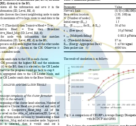
The assumed parameters used in the simulations are summarized in table 1.
Table 1 Simulation parameters
Parameter Value
Network field (0, 0)–(100,100) m Base station location (150, 100) m N (Number of nodes) 100 Initial energy (EInit) 1 J Eelec (E.Dissipation for ETx & ERx) 50 nJ/bit ε fs (free space) 10 pJ/bit/m2 ε mp (Multipath fading) 0.0013 pJ/bit/m4 do (Threshold distance) 87 m EDA (Energy Aggregation Data) 5 nJ/bit/signal Data packet size (l) 4000 bits
The result of simulation is as follows:
Fig.3. A comparison of CELRP's Average Energy Dissipation with BCDCP and GPRS
rounds of CELRP is higher than BCDCP and GPRS. So CELRP has better performance than BCDCP and GPRS in terms of energy efficiency as well as able to prolong network lifetime of sensor node.
Fig.4. A comparison of CELRP's system lifetime With BCDCP and GPRS
Fig. 4 clearly shows that the number of lifetime of nodes (the numbers of live sensor nodes until the first node dies) for CELRP is higher over BCDCP and GPRS. The life time starts decreasing at round 150 in BCDCP and at round 200 for GPRS, while in the case of CELRP the decrease only starts after more than 360 rounds. Compared to CELRP, we calculated that in BCDCP the node died 29% faster and in GPRS the node died 17% faster than the CELRP. That means an average number of live sensor nodes in CELRP is 29% higher than BCDCP and 17% higher than GPRS. Therefore it has been clearly shown that CELRP is better in prolonging network lifetime and balancing energy consumption compare to the BCDCP and GPRS. It should also be noted that the graph of CELRP is smoother than the BCDCP and GPRS.
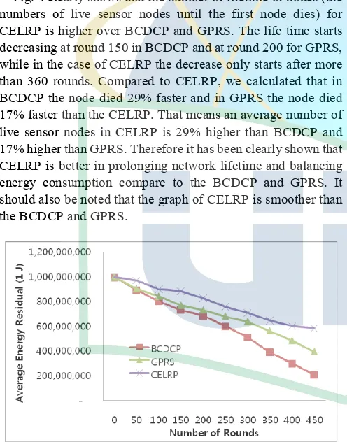
Fig 5. A comparison of CELRP's Average Residual Energy with BCDCP and GPRS
Fig. 5 shows the average Residual Energy over the number of rounds. CELRP significantly reduces energy consumption compared to BCDCP and GPRS because CELRP uses an alternative method that selects the CH based on its’ location and
measurement of Residual Energy. The method of division into quadrants and the use of multi hop for transmission data in each cluster also resulted in a more efficient energy usage and less consumption of energy for both intra and inter cluster data transmission in CELRP. The reduction in average energy residual can be obtained by 22% higher than BCDCP and 10% than GPRS which means that the CELRP consumes about 22% less energy than BCDCP and 10% less than GPRS. The graphs curve shows that the dissipation that varied between rounds of CELRP is higher than BCDCP and GPRS. So CELRP has better performance than BCDCP and GPRS in terms of energy efficiency as well as able to prolong network lifetime of sensor node.
Fig 6. A Network Lifetime as The Base Station Travels Farther
Fig. 6 Study impact the distance to the Base Station on the network lifetime. We fix the y* coordinate of the Base Station and adjust its x *coordinate. The distance is computed from the Base Station to the closest point of the network field. Under the setting of the distance an optimum TD_MAX is chosen to extend the network lifetime. We measure the number of rounds until the first node dies in CELRP, GPRS and BCDCP; the result shown in Fig 5. Although the network lifetime severally deteriorates as the distance increases, CELRP achieves about 1.1 x network lifetimes as the distance increases than GPRS and achieves about 2.3 x network lifetime as distance increase than BCDCP for all the Base Station location we simulated.
VII. CONCLUSION
We assumed that the Base Station has all the information including the sensor nodes, the residual energy and the distance of node that have been defined. All the results from simulations shown and proved that the network lifetime and balanced energy consumption of A Cluster Based Energy Efficient Location Routing Protocol (CELRP) in Wireless Sensor Networks are better than that of the BCDCP and GPRS when compared in large area network. The simulation results proved that a Cluster Based Energy Efficient Location Routing Protocol (CELRP) in Wireless Sensor Networks is highly energy efficient, and can prolong network lifetime and balances energy consumption.
REFERENCES
[1] B. Karp and H. T. Kung. GPSR: greedy perimeter stateless routing for wireless networks. In IEEE/ACM MOBICOM, 2000, pp. 243–254. [2] B. Karp and H. T. Kung, "GPSR: Greedy Perimeter Stateless Routing for
Wireless Networks,” MobiCom 2000.
[3] E. Kranakis, H. Singh, and J. Urrutia, "Compass Routing on Geometric Networks," Proc. 11th Canadian Conf. Computational Geometry, Aug.1999
[4] H. Sabbineni and K. Chakrabarty. Location*aided flooding: an energy efficient data dissemination protocol for wireless sensor networks. IEEE Transactions on Computers, 2005, 54:36–46.
[5] H. Shen, “Finding the k Most Vital Edges with Respect to Minimum Spanning Tree,” in Proceedings of IEEE Nat’l. Aerospace and Elect. Conf., vol. 1, 1997, pp. 255*262.
[6] J. Gao, L. J. Guibas, J. Hershberger, L. Zhang, and A. Zhu. Geometric spanners for routing in mobile networks. IEEE Journal on Selected Areas in Communications, 2005, 23.174–185.
[7] J. Li, J. Jannotti, D. DeCouto, D. Karger, and R. Morris. A scalable location service for geographic ad*hoc routing. In IEEE/ACM MOBICOM, 2000, pp. 120–130.
[8] Jazyah Y. and Hope M. D. “A New Routing Protocol for UWB MANET, proceeding of the 10th WSEAS International Conference on Eroupean Conference System (ECS’10), and Signal Processing, Cambridge, UK, February 2010, pp.24 – 28.
[9] J. N. Al*Karak and A. E.Kamal, "Routing techniques in wireless sensor network: A survey” .IEEE wireless communications, Vol. 11, pp. 6*28, December 2004
[10] Ming*Jer Tsai, hong*yen yang,bing*Hong liu and Wen*Qian huang. Virtual*Coordinat A Geography*based Heterogeneous Hierarchy Routing Protocol in Wireless Sensor Networks. INFOCOM, 2008, pp. 351–355, [11] . D. Muruganathan, D. C. F Ma., R. I. Bhasin, and A. O. Fapojuwo, “A Centralized Energy*Efficient Routing Protocol for Wireless Sensor Networks,” IEEE Communications Magazine, vol.43, 2005, pp. 8*13. [12] S. Lee, B. Bhattacharjee, and S. Banerjee. Efficient geographic routing in
multihop wireless networks. In IEEE/ACM MOBIHOC, 2005, pp. 230–24.
[13] S. Ratnasamy, B. Karp, L. Yin, F. Yu, D. Estrin, R. Govindan, and S. Shenker. GHT: a geographic hash table for data*centric storage. In ACM WSNA, 2002, pp. 78–87.
[14] W. B. Heinzelman, A. P. Chandrakasan, and H. Balakrishnan, “Energy Efficient Communication Protocol for Wireless Microsensor Networks,” in Proceedings of 33rd Hawaii Int’l. Conf. Sys. Sci., 2000.
[15] W. B. Heinzelman, A. P. Chandrakasan, and H. Balakrishnan, “An Application*Specific Protocol Architecture for Wireless Microsensor Networks”, IEEE Transactions on Wireless Communications, vol.1, Oct. 2002, pp. 660*670.
[16] W. B. Heinzelman, “Application*Specific Protocol Architectures for Wireless Networks,” Ph.D. Thesis, Massachusetts Institute of Technology (MIT), June 2000.
[17] W. Heinzelman, A. Chandrakasan and H. Balakrishnan, An application*specific protocol architecture for wireless micro sensor networks, IEEE Transactions on Wireless Communications 1(4), 2005, pp. 660–670
[18] W. H. Liao, Y. C. Tseng, and J. P. Sheu, "GRID: A fully location*aware routing protocols for mobile ad hoc networks," Proc. IEEE HICSS, January 2000.
[19] Xi. Chen, Honglian Ma and Keqiu Li. A Geograhpy*based Heterogeneous Hierarchy Routing Protocol Wireless Sensor Networks IEEE International Conference on High Performance computing and communications, 2008, pp. 767–774.
[20] Xin Su, Dongmin Choi. and et al., “An Energy*Efficient Clustering for Normal Distributed Sensor Networks”, Proceedings of the9th WSEAS International Conference on VLSI and Signal Processing (ICNVS’10), Cambridge, UK, February 2010, pp.81 – 84
[21] Y. B. Ko and N. H. Vaidya, "Location*Aided Routing (LAR) in mobile ad hoc networks," Wireless Networks 6 (2000) 307–321 307.
[22] Yih*Jia Tsai and Chen*Han Yao, ‘Local Recovery Routing Protocol with Clustering Coefficient’ New Aspects of Applied Informatics, Biomedical Electronics & Informatics and Communications, , Proceeding 10th WSEAS International Conference on applied Informatics and Communications (AIC’10),Taipei, Taiwan August 20*22, 2010, pp. 64 * 68
[23] Young Han Lee, Kyoung Oh Lee. and et al. CBERP: Cluster Based Energy Efficient Routing Protocol for Wireless Sensor Network. Recent Advances in Networking, Proceeding of the 12th WSEAS International Conference on VLSI and Signal Processing (ICNVS’10), Cambridge, UK, February 2010, pp.24 * 28.
[24] Y. Zou and K. Chakrabarty. A distributed coverage*and connectivity centric technique for selecting active nodes in wireless sensor networks. IEEE Transactions on Computers, 2005, 54:978–991.H. Poor, An Introduction to Signal Detection and Estimation. New York: Springer*Verlag, 1985, ch. 4.
was born 1969 and obtained her Bachelor’s Degree in informatics engineering and management in 1994 from Gunadarma University, Jakarta Indonesia, and Master Degree in computer science in 2003 from University of Indonesia, majoring information technology, Jakarta, Indonesia.
She is now PhD student in Sun Moon University, South Korea, and current research interest in Routing Protocol in Wireless Sensor Networks.
Nurhayati is member of Korea Information Processing Society.
was born 1953, November 9 and obtained his Bachelor Science Degree in mathematics in 1977 from Sogang University, Seoul, Korea and Master Science Degree in computer science in 1988 from Pennsylvania University, University Park, PA, USA and PhD in computer science in 1994 from University of Kentucky, Lexington, KY, USA, 1994.
He is Professor in Sun Moon University, Asan, Chung*nam, Korea in 1995 until now and current research interest in Computational Complexity, Numerical Analysis. Prof. Sung Hee Choi is member of Korea Information Society