Test Generation Algorithm Based on SVM with
Compressing Sample Space Methods
Ting Long*1, Jiang Shiqi1, Hang Luo2 1
School of Control Engineering, Chengdu University of Information Technology, Chengdu, 610225, China
2
School of Manufacturing Science and Engineering, University of Sichuan, Chengdu, 610065, China *Corresponding author, e-mail: [email protected]1, [email protected]2
Abstract
Test generation algorithm based on the SVM (support vector machine) generates test signals derived from the sample space of the output responses of the analog DUT. When the responses of the normal circuits are similar to those of the faulty circuits (i.e., the latter have only small parametric faults), the sample space is mixed and traditional algorithms have difficulty distinguishing the two groups. However, the SVM provides an effective result. The sample space contains redundant data, because successive impulse-response samples may get quite close. The redundancy will waste the needless computational load. So we propose three difference methods to compress the sample space. The compressing sample space methods are Equidistant compressional method, k-nearest neighbors method and maximal difference method. Numerical experiments prove that maximal difference method can ensure the precision of the test generation.
Keywords: Test Generation, SVM (Support Vector Machine), k-nearest Neighbors, Maximal Difference
1. Introduction
A recent trend in analog test strategies is called test generation. It can establish convenient signals to excite the input of the device under test (CUT), observe the response [1], and decide whether the CUT is faulty based on the response [2]-[12]. The analog test generation is different from the digital test generation [13],[14].
Fault detection and classification in this paper are based on a Support Vector Machine (SVM), so that the response vectors of normal and faulty circuits can be distinguished on the basis of nonlinear classification. SVM [15],[16] is to classify small samples based on statistical learning theory. This method has proven adept at dealing with highly nonlinear classification problems. The rule-less response data sampled from electronic systems are an excellent example. When the bandwidth of the DUT is much smaller than the sampling frequency of the DAC/ADC, the sample vectors of the impulse-response become quite large. The response data of the sample space contains redundant data, because successive impulse-response samples may get quite close. The redundancy will waste the needless computational load. In this paper we propose a maximal difference method to compress the sample space, and reduce computational load.
2. Test generation algorithm
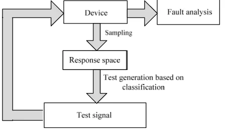
An analog DUT can be treated as a discrete time digital system by placing it between a digital-to-analog converter (DAC) and an analog-to-digital converter (ADC) [12]. Many circuit instances, which are either normal or given parametric faults, must be simulated for the test generation. Each instance is labeled as ‘passed’ or ‘failed’. A passed instance means that the simulated parameters match their specifications. A failed instance means that the simulated parameters do not match their specifications. A response vector is constructed for each circuit instance by sampling the analog output signal [12]. So we can sample the output response of a passed or failed instance to represent the circuit. Then the sample space can be obtained from many circuit instances. This space will be used as training set or testing set [17]-[19] for classification in the test generation.
Figure 1. Process of the test algorithm based on SVM
The classification hyperplane determined for the output response space is the same as that determined for the impulse-response space [12]. Thus, we can also obtain the simulated parameter sets by sampling the impulse responses of the circuit instances. The simulated parameter sets can themselves be considered output vectors, and used to build the sample space.
Sv=(S[0], S[1], S[2],···) is a sample vector for one impulse response. Many such vectors construct the sample space (Sv1, Sv2, Sv3, ···). However, the output response mainly comes from the range S = (s[0], s[1],···, s[d−1]), where d=Fs/BW and BW is the bandwidth of the LTI. So impulse-response sample space (S1, S2,···, Si,···) is constructed by S-vectors.
In the analysis of some analog systems the responses of normal circuits are similar to those of circuits with small parametric faults, so the response vectors are mixed together. It is difficult to classify the sample space constructed by these response vectors with any existing test generation algorithm. A SVM can deal with this sample space by mapping it to a higher-dimensional feature space and separating the groups with a hyperplane. We can use SVM for the test generation to execute the classification process, and obtain the test signals from the classification hyperplane.
The optimal hyperplane algorithm proposed by Vladimir Vapnik was a linear classifier. Reference [20] proposed a way to create nonlinear classifiers by applying the kernel functions to maximum-margin hyperplanes.
We obtain support vectors from the training set with the SVM algorithms [21]. The hyperplane can be built from the support vectors.
S
Tis the transpose ofS
. The test signals can then be calculated by the optimal hyperplane as the test sequence.3. Compression of the sample space 3.1. Equidistant compressional method
When the bandwidth BW of the DUT is much smaller than the sampling frequency Fs of the DAC/ADC, the sample vectors of the impulse-response become quite large considering d=Fs/BW. Then the sample space of the impulse-response becomes quite large too. This sample space contains redundant data, because successive impulse-response samples may get quite close. The redundancy will waste the needless computational load. For reducing computational load, a small number of impulse-response samples can be extracted from the vector H to build the new sample space. So the compression of the sample space means decreasing the length of every sample vector.
Reducing the length of a sample vector always decreases the cost of the calculation, but may imply a loss of information. So before decreasing the sample space, we must ensure that the remaining information suffices for the classification. In this paper, we require that the efficiency of the test remains satisfactory, meaning that the parameters generated by the test algorithm are effective. The efficacy of the test is dependent on the precision of the classification.
vector after extracting samples from H = (s[0], s[1],···, s[d−1]) with distance 4. This method is easy to be executed. But it cannot ensure that the remaining information suffices for the classification, when the length of every new sample vector is very small, because the extracted s[i] for the new sample vectors is not always the most effective for classification in this method.
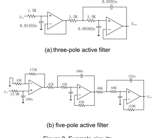
We use the circuits in Figure 2 to show the results of the equidistant compressional method, and assign normal and faulty parameters to the components in Figure 2 to build normal and faulty circuit instances. All the parameters fall inside their respective ranges of tolerance in normal circuit.
We can construct a sample space with sample vectors from the circuit shown in Figure 2. A sample vector, which length is set to 30, is obtained by sampling the impulse response of a circuit instance. It can be written as (s[0], s[1],···, s[28], s[29]). In the training set, each sample vector is labeled as ‘passed’ or ‘failed’ according to the circuit specifications. The testing set classifications are derived by comparing the output response to a threshold derived from the hyperplane coefficients, following the test generation method based on SVM.
Vin
Table 1 shows the misclassification rates for the circuits in Figure 2 by the test generation algorithm based on SVM. For the passed (failed) population, the misclassification is defined as the ratio between the number of correctly classified passed (failed) instances to the number of instances labeled as passed (failed). The test generation method based on SVM implemented in this paper achieves low misclassification rates.
Table 1. Misclassification Rates of Test Generation based on SVM for Figure 2
Misclassification
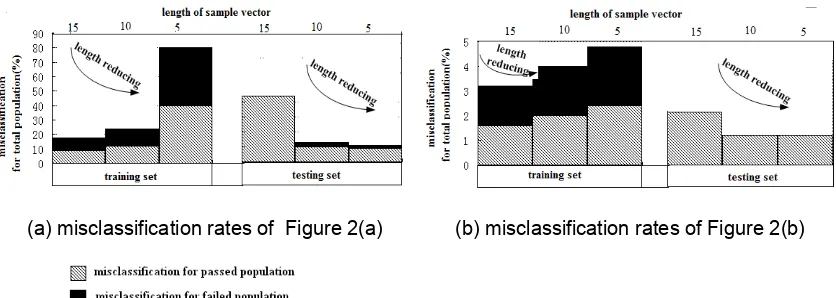
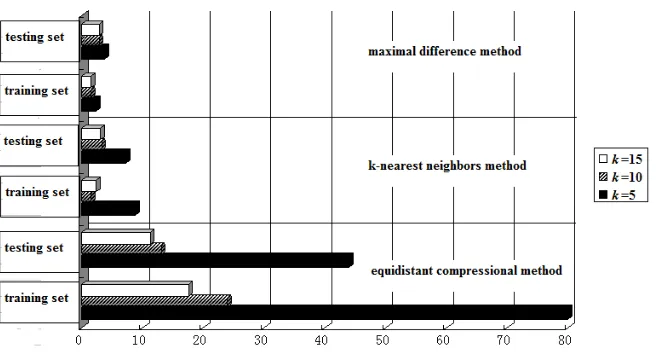
length of every impulse-response sample vector. We use k to represent the length of the new sample vector after extracting samples. If k=15, the sample vector would be(s[1], s[3],···, s[27], s[29]). We could also construct the sample vectors (s[2], s[5],···, s[26], s[29]) and (s[4], s[9], s[14], s[19], s[24], s[29]) with k=10 and k=5 samples respectively. Figure 3 shows the misclassification rates for the circuits of Figure 2, with different values of k. The misclassification rates for passed and failed population are denoted in Figure 3 by different bars. The sum of the misclassification rates for passed and failed population means the misclassification rate for total population.
Figure 3(b) shows that the misclassification rates for the total training or testing set of Figure 2(b) for k=15, k=10 and k=5 respectively. Consulting the misclassification rates in Table 1, the effect of reducing the length of every sample vector is acceptably small, and the equidistant compressional method is useful even for sample vectors of low dimension.
But for the circuit of Figure 2(a), Figure 3(a) shows that the misclassification rates for the totaltraining and testing set can achieve 80% and 44% when we reduce the length of every sample vector. The misclassification rates are very high, and cannot be accepted. So for Figure 2(a) the equidistant compressional method is disabled. Because the new sample vectors are not the most effective for classification.
(a) misclassification rates of Figure 2(a) (b) misclassification rates of Figure 2(b)
Figure 3. Misclassification rates for different values of k by equidistant compressional method
In the following sections we will propose two other different methods to compress the sample space, and contrast the three methods. We will show the best method for compression of sample space by the extensive experiment results.
3.2. k-nearest neighbors method
In this section we will propose a method to compress the impulse-response sample space based on k-nearest neighbors algorithm.
Suppose that an impulse-response sample space is (S1,···Sn, Sn+1, ···Sm). In this sample space the number of impulse-response sample vectors labeled as ‘passed’ is n, and the number of impulse-response sample vectors labeled as ‘failed’ is m-n. Hi which is (si[0], si[1],···,
si[d-1]) (i=1,···n, n+1,···m) denotes one impulse-response sample vector. The original length of
The k-nearest neighbors algorithm is a useful method for pattern classification [22]. The testing set here is the target set for classification. For one sample in the testing set, this method can be run in the following steps:
1) For this sample, locate the t nearest samples of the training set. t is the number of the nearest samples.
2) Examine that most of the t nearest samples belong to which category of the training set.
3) Assign this category to this sample in the target dataset.
A Euclidean distance measure is used to calculate how close each sample of the testing set is to the training set. Given sx = (sx1,sx2,..., sxn) which is a sample in the testing set
So k-nearest neighbors method classifies the testing set based on the class of their nearest neighbors. It can be executed fast for the low-dimensional space. So it can be used to execute the classification for Pj .
The compressional method of the impulse-response sample space based on k-nearest neighbors algorithm can be run in the steps as follows:
1) Calculate the misclassification rate for each Pj with k-nearest neighbors algorithm. 2) Based on the misclassification rates obtained by step 1), select k Pjs with low misclassification rates to construct the new sample space.
Then the new sample space can be used to the test generation.
The k-nearest neighbors method is a classification method here. The crucial problem for all the classification methods is to reduce misclassification rates. When the misclassification rates are too high, we must find other methods to reduce them. It makes the k-nearest neighbors method complex to apply to compress the sample space. The next section will present another method to compress the sample space without the classification.
3.3. Maximal difference method
In this section we will propose another method to compress the impulse-response sample space based on maximal difference of the categories. It’s called the maximal difference method.
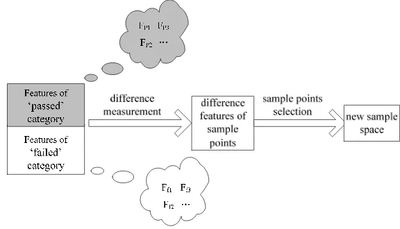
We use the impulse-response sample space (S1,···Sn, Sn+1, ···Sm) which was illustrated in last section to show the maximal difference method. The method just utilizes the training set for compression. It can be run in the steps of Figure 4.
The features of ‘passed’ or ‘failed’ category are the average values in the training set. Use vector Fp =(Fp1, Fp2, Fp3,···) to represent the feature of ‘passed’ category, and vector Ff =(Ff1, Ff2, Ff3,···) to represent the feature of ‘failed’ category.
The difference features of sample points are obtained by measuring the distances of Fp and Ff . The maximal difference method selects the maximal features to construct the new sample space.
3.4. Comparison
We use different methods to compress sample space of impulse-response. These methods are equidistant compressional method, k-nearest neighbors method and maximal difference method. Figure 5 shows that the sample points of the compressed sample space of impulse-response. The equidistant compressional method is to extract samples with invariable distance. So the new sample vectors of the compressed sample space for the circuits of Figure 2 are alike.
(a) sample points of Figure 2(a) when k=15 (b) sample points of Figure 2(a) when k=10
(c) sample points of Figure 2(a) when k=5 (d) sample points of Figure 2(b) when k=15
Figure 5. Sample points of the compressed sample space of impulse-response from different methods
Contrast to the k-nearest neighbors method and the maximal difference method, the k-nearest neighbors method is a classification method. This method is more complex than the maximal difference method. The maximal difference method only needs to calculate the average values of each category, and doesn’t need to consider the testing set. It is not a classification method, and doesn’t need to recognize the two categories. So it is not a complex classification process. The computational process of it is simpler than the k-nearest neighbors method. So we can choose it for the compression of the sample space if its misclassification rates are low enough for the test.
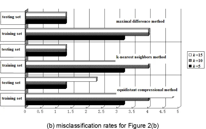
The misclassification rates for the different compressional methods are illustrated in Figure 6. We compare the three compressional methods presented by Figure 6. For example, Figure 6(a) shows the misclassification rates for Figure 2(a) when k=15, 10 and 5. So according to the misclassification rates in Figure 6 the k-nearest neighbors method is more effective than the equidistant compressional method, and the maximal difference method is more effective than the k-nearest neighbors method.
So considering the complexity of the computational process and the misclassification rates, the maximal difference method is the best choice for the compression of the sample space.
(b) misclassification rates for Figure 2(b)
Figure 6. Misclassification rates for different compressional methods
4. Conclusions
In this paper we have proposed an effective test generation algorithm for analog circuits with compressing sample space methods. The algorithm uses a SVM to obtain the test signals.
For the compression of the sample space we contrast three compressional methods, including equidistant compressional method, k-nearest neighbor’s method and maximal difference method. Considering the complexity of the computational process and the misclassification rates, we can choose the maximal difference method as the compressional method. The experiments can prove the efficiency of the maximal difference method.
References
[1] Ke H, Stratigopoulos HG, Mir S, Hora C, Yizi X, Kruseman B. Diagnosis of Local Spot Defects in Analog Circuits. IEEE Transactions on Instrumentation and Measurement. 2012; 61(10): 2701-2712. [2] Cheng LY, Jing Y, Zhen L, Shulin T. Complex Field Fault Modeling-Based Optimal Frequency
Selection in Linear Analog Circuit Fault Diagnosis. IEEE Transactions on Instrumentation and
Measurement. 2014; 63(4): 813-825.
[3] Ahmadyan SN, Kumar JA, Vasudevan S. Goal-oriented stimulus generation for analog circuits. 49th Design Automation Conference. 2012; 6: 1018-1023.
[4] Ozev S, Orailoglu A. An integrated tool for analog test generation and fault simulation. International Symposium on Quality Electronic Design. 2002: 267-272.
[5] Voorakaranam R, Chatterjee A. Test generation for accurate prediction of analog specifications. 18th IEEE VLSI Test Symposium. 2000; 5: 137-142.
[6] Huynh SD, Seongwon K, Soma M, Jinyan Z. Automatic analog test signal generation using multi-frequency analysis. IEEE Transactions on Circuits and Systems II: Analog and Digital Signal
Processing. 1999: 565- 576.
[7] Qi ZZ, Yong LX, Xi FL, Dong JB, Xuan X, San SX. Methodology and Equipments for Analog Circuit Parametric Faults Diagnosis Based on Matrix Eigenvalues. IEEE Transactions on Applied
Superconductivity. 2014; 24(5):0601106.
[8] Cauwenberghs G. Delta-sigma cellular automata for analog VLSI random vector generation. IEEE
Transactions on Circuits and Systems II: Analog and Digital Signal Processing. 1999; 46(3): 240-250.
[9] Zheng HH, Balivada A, Abraham JA. A novel test generation approach for parametric faults in linear analog circuits. 14th Proceedings of VLSI Test. 1996; 5: 470–475.
[10] Soma M. Automatic test generation algorithms for analogue circuits. IEE Proceedings Circuits, Devices and Systems. 1996: 366-373.
[11] Fuh LW, Schreiber H. A pragmatic approach to automatic test generation and failure isolation of analog systems. IEEE Transactions on Circuits and Systems. 1979; 26(7): 584-585.
[12] Chen YP, Kwang TC. Test generation for linear time-invariant analog circuit. IEEE Transactions on
Circuits and Systems II: Analog and Digital Signal Processing. 1999; 46(5): 554-564.
[13] Yu W, Hao W, Zhenyu S. A Prioritized Test Generation Method for Pairwise Testing. TELKOMNIKA
[14] Liu X. Learning Techniques for Automatic Test Pattern Generation using Boolean Satisfiability.
TELKOMNIKA Indonesian Journal of Electrical Engineering. 2013; 11(7): 4077-4085.
[15] Vapnik VN. Overview of statistical learning theory. IEEE Transactions on Neural Networks. 1999; 10(5): 988-999.
[16] Vapnik V. SVM method of estimating density, conditional probability, and conditional density. IEEE International Symposium on Circuits and Systems. 2000; 2: 749-752.
[17] Richard OD, Peter EH, David GS. Pattern classification. Wiley-Interscience. 2000: 11.
[18] Yan HF, Wang WF, Liu J. Optimization and application of support vector machine based on SVM algorithm parameters. Journal of Digital Information Management. 2013; 11(2): 165-169.
[19] Demetgul, Mustafa, Yazicioglu O, Kentli A. Radial basis and LVQ neural network algorithm for real time fault diagnosis of bottle filling plant. Tehnicki Vjesnik. 2014; 21(4): 689-695.
[20] Huang TM, Kecman V, Kopriva I. Kernel Based Algorithms for Mining Huge Data Sets, Supervised,
Semi-supervised, and Unsupervised Learning. Springer-Verlag, Berlin, Heidelberg. 2006: 96-97.
[21] Ting L, Houjun W, Bing L. Test generation algorithm for analog systems based on support vector machine. Signal, Image and Video Processing. 2011; 5(4): 527-533.
[22] T Cover, P Hart. Nearest neighbor pattern classification. IEEE Transactions on Information Theory.