EVIDENCE FROM INDONESIAN STOCK MARKET
KALEEM SALEEM
GRADUATE SCHOOL
BOGOR AGRICULTURAL UNIVERSITY
BOGOR
I do hereby declare that the thesis entitled "ANALYSIS OF PORTFOLIO
OPTIMIZATION WITH AND WITHOUT SHORTSELLING BASED ON
DIAGONAL MODEL: EVIDENCE FROM INDONESIAN STOCK MARKET" is
my original work produced through the guidance of my academic advisors and that to the best of my knowledge it has not been presented for the award of any degree in any educational institution. All of the incorporated material originated from other published as well as unpublished papers are clearly stated in the text as well as in the references.
Hereby I delegate the copy rights of this work to the Bogor Agricultural University. Bogor, October 2013
Kaleem Saleem
KALEEM SALEEM. Analysis of Portfolio Optimization with and without Shortselling based on Diagonal Model: Evidence from Indonesian Stock Market.
Supervised by ABDUL KOHAR IRWANTO dan ENDAR HASAFAH
NUGRAHANI.
Markowitz (1952, 1959) and Roy (1952) proposed portfolio theory which narrate that risk of a portfolio is the variance of individual securities and covariances among those securities comprising the portfolio. The objectives of this research is to construct an optimized portfolio using Sharpe's diagonal model with and without short selling respectively, and to analyze the performance of less diversified optimal portfolios by investing in a single industry versus well diversified portfolio by investing across all industries. Finally to analysis the statistical properties of the estimates of diagonal model.
Markowitz mean-variance portfolio optimization theory is implemented for all stocks listed in 9 sectors of Indonesian stock market during 2007-2011. However our model used 269 stocks which are not contradicting to the basic assumptions of the diagonal model. Diagonal model used in this research is a linear model and data used are time series secondary data. Firstly 9 optimal portfolios are computed for individual sectors with the assumption that short selling not permitted and then computation is done with assumption that short selling is permitted. Similarly 2 optimal portfolios are computed consisting of all stocks with assumptions mentioned above.
Results showed that both well diversified short and long portfolios provide higher returns at a specified risk level compare to portfolios consist of individual sectors stocks. Largest weight in short portfolio is from infrastructure, utilities and transportation sector equaling 17.2 percent. Largest weight in long only portfolio are from trade, investment and services sector equaling 23.2 percent. The more diversified and larger portfolios provide better tangency portfolio. All stocks short and long portfolios performed better than any other individual sector portfolio. Standard error for β and residual standard error for other portfolios are large compare to individual stocks indicating risk was not diversified away. Least square parameters estimates were not quite promising such as value of portfolio beta happened to be less than individual stocks as well as value of its coefficient of determination shows most of the systematic risk could not get eliminated as low values of R2
for portfolios shows that most of the variance in stock return as well as in portfolio return is not explained by market variance therefore unsystematic risk could not get eliminated despite of forming a portfolio encompassing all equities listed in Indonesian Stock Exchange as suggested by results of regression analysis.
KALEEM SALEEM. Analisis Optimisasi Portofolio dengan dan tanpa Shortselling bardasarkan Diagonal Model: Bukti dari Pasar Saham Indonesia. Dibimbing oleh ABDUL KOHAR IRWANTO dan ENDAR HASAFAH NUGRAHANI.
Markowitz (1952 , 1959) dan Roy (1952) mengusulkan teori portofolio yang menceritakan bahwa risiko portofolio adalah varians dari sekuritas individual dan covariances antara mereka. Tujuan dari penelitian ini adalah untuk membangun sebuah portofolio optimal menggunakan model diagonal Sharpe dengan and tanpa short selling berturut-turut, dan untuk menganalisis kinerja portofolio optimal yang kurang terdiversifikasi dengan berinvestasi di portfolio industri individu dibandingkan portofolio yang terdiversifikasi dengan berinvestasi di semua industri. Akhirnya menganalisis sifat statistik perkiraan model diagonal .
Markowitz teori mean-variance diterapkan untuk semua saham yang tercatat di 9 sektor pasar saham Indonesia selama 2007-2011. Namun model kami menggunakan 269 saham yang tidak bertentangan dengan asumsi dasar dari model diagonal. Model diagonal digunakan dalam penelitian ini adalah model linier dan data yang digunakan adalah data time series sekunder. Pertama 9 portofolio optimal dihitung untuk masing-masing sektor dengan asumsi bahwa short selling tidak diperbolehkan dan kemudian dengan asumsi bahwa short selling diperbolehkan. Demikian 2 portofolio optimal dihitung terdiri dari semua saham dengan asumsi tersebut di atas.
Hasil penelitian menunjukkan bahwa kedua terdiversifikasi portofolio short dan long memberikan hasil yang lebih tinggi pada tingkat risiko tertentu dibandingkan dengan portofolio terdiri dari saktor saham individu. Bobot terbesar di portofolio short adalah dari infrastruktur , utilitas dan sektor transportasi setara 17,2 persen. Bobot terbesar di portofolio long adalah dari sektor perdagangan, investasi dan jasa setara 23,2 persen. Portofolio lebih beragam dan lebih besar menyediakan portofolio singgung yang lebih baik. Semua saham portofolio short dan long dilakukan lebih baik daripada portofolio sektor individu lain. Standar error untuk β dan residual standar error untuk portofolio lainnya besar dibandingkan dengan saham individu yang menunjukkan risiko tidak didiversifikasi. Least square perkiraan parameter tidak cukup menjanjikan seperti nilai portofolio β kebetulan kurang dari saham individu serta nilai koefisien determinasi menunjukkan sebagian besar risiko sistematis tidak bisa mendapatkan dieliminasi sebagai nilai-nilai rendah R2
untuk portofolio menunjukkan bahwa sebagian besar dari varians dalam return saham serta return portofolio tidak dijelaskan oleh varians pasar sehingga risiko tidak sistematis tidak bisa mendapatkan dihilangkan meskipun membentuk portofolio meliputi semua saham yang terdaftar di Bursa Efek Indonesia seperti yang disarankan oleh hasil analisis regresi.
No part or all of this work may be excerpted without inclusion or mentioning the sources. Exception only for research and education use, writing for scientific papers, reporting, critical writing or reviewing of a problem; and this exception does not inflict a financial loss in the proper interest of Bogor Agricultural University.
EVIDENCE FROM INDONESIAN STOCK MARKET
KALEEM SALEEM
A Thesis submitted in partial fulfillment of the requirements for the award of the degree Master of Science
in Management
GRADUATE SCHOOL
BOGOR AGRICULTURAL UNIVERSITY
BOGOR
Name : Kaleem Saleem
NRP : H251118101
Approved by
Advisory Committee
Dr Ir Abdul Kohar Irwanto, MSc Dr Ir Endar Hasafah Nugrahani, MS
. Supervisor Co-supervisor
Agreed by
Program Coordinator Dean of Graduate School
Management Science
Dr Ir Abdul Kohar Irwanto, MSc Dr Ir Dahrul Syah, MScAgr
I would borrow few sentences to praise God Almighty Allah SWT, and Our Lord Mohammad SAW from Richard Burton's translation of 'The Arabian Nights', "Praise be to Allah, The Beneficient King, The Creator of The Universe, Lord of the Three Worlds, who set up the firmament without pillars in its stead, and who stretched out the earth even as a bed, and grace and prayer-blessing be upon our Lord Mohammed, Lord of Apostolic Men, and upon His family and companion".
I would like to express my deepest gratitude and thanks to the Indonesian taxpayers for financing my postgraduate studies at Bogor Agricultural University in Indonesia and was deeply honored to receive the Indonesian Government Postgraduate Scholarship for Developing Countries which enabled me to pursue advance studies in management science. This research is also made possible by funding from Bureau of Planning and International Cooperation, Ministry of National Education of The Republic of Indonesia and author is extremely grateful to the ministry for this generosity.
This work could not be made possible without the supervision, support and constant guidance of my supervisors Dr Ir Abdul Kohar Irwanto MSc and Dr Ir Endar Hasafah Nugrahani MS. I am highly grateful to them for this kindness. I am also thankful to Dr Mukhlis Ansori MSc for his lessons of Bahasa Indonesia. Without the firm support and prayers of my beloved parents Dr Muhammad Saleem Baloch and Zubaidah Baloch and my beloved family Parigul, Shahgulee, Fauziah, Faheem, Saimah, Waseem and Hassam this milestone could never be accomplished. I am also grateful to my classmates Jonathan, Roto, Didu, Budi, Mita, Nunung, Hamadani, Ajen, Dani, Yanti, Jay, Dewi, Arfan and to all of them whose names are not mentioned here. Finally I am extremely indebted to Jazirotul and Adek Aruna, Dr Adil, Wahidullah, Dr Walter, Petlane, Princy, Constantine, Hagim, Hirmawan, Ujang, Pungki, Pak Soleh Hidayat, Gani, Sinath, Faye, Andrew, Chris, Fredrik, Aziz, Sari, Isma, Viladmir, Musa and whole KNB family for their enormous support during all these years in Indonesia. Last but not the least I am extremely thankful to Indonesia itself, I have experienced living in one of the most beautiful places on planet, with surprisingly wonderful and friendly people. Indonesia is no doubt a piece of paradise on earth.
Bogor, October 2013
TABLE OF CONTENTS vii
LIST OF FIGURES x
LIST OF TABLES xii
LIST OF APPENDICES xiv
1 INTRODUCTION 1
1.1 Background 1
1.2 Problem Formulation 2
1.3 Research Objectives 2
1.4 Research hypothesis 3
1.5 Research Benefit 3
2 LITERATURE REVIEW 4
2.1 Emergence of Modern Portfolio Theory 4
2.2 Overview of Indonesian Stock Market 5
2.3 Choices Under Certainty 6
2.4 Mean and Variance 7
2.5 Mean, Variance and Covariance of Portfolio 8
2.6 Diversification 9
2.7 Portfolio Possibilities Curve 10
2.8 One Fund Theorem 13
2.9 Portfolio Optimization with Quadratic Programming 14
2.10 Single Index Model 17
2.11 Previous Researches 20
3 METHODOLOGY 23
3.1 Research Framework 23
3.2 Diagonal Model 23
3.3 Research Method 24
3.4 Research Limitations 25
3.5 Data 26
3.6 Portfolio Optimization with R 26
4 RESULTS & DISCUSSION 29
4.1 Agriculture Sector 29
4.2 Mining Sector Portfolio 33
4.3 Basic Industry & Chemicals Sector Portfolio 37
4.4 Miscellaneous Industry Sector Portfolio 41
4.5 Consumer Goods Industry Portfolio 45
4.6 Property, Real Estate and Building Construction Portfolio 49 4.7 Infrastructure, Utilities and Transportation Portfolio 53
5 CONCLUSION 73
6 RECOMMENDATIONS 73
REFERENCES 74
1 Consumption in period 1 and period 2 for a single asset with certain
outcomes 6
2 Consumptions in period 1 and 2 for multiple assets with certain outcomes 7 3 Perfectly positive covariance between asset A and asset B 10 4 Perfectly negative covariance between asset A and asset B 11
5 Zero covariance between asset A and asset B 12
6 Combination of riskless asset with risky assets 14
7 Maximum value ofθwhen dXdθ
i <0at maximum feasible value ofθ
whenXi = 0 16
8 Maximum value ofθwhen dXdθ
i = 0at maximum feasible value ofθ
whenXi = 0 17
9 β is shown by the slope of line 19
10 Return Plot during 2007-2011 29
11 Efficient Frontier Optimal Portfolio Agriculture Sector 30
12 Performance Chart Agriculture Portfolio 33
13 Efficient Frontier Optimal Portfolio Mining Sector Sector 34
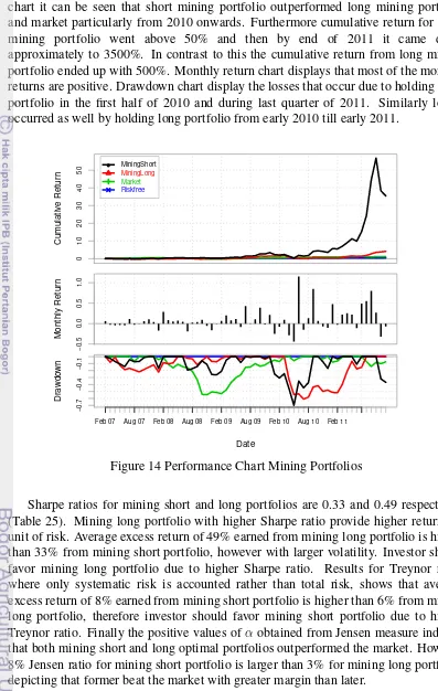
14 Performance Chart Mining Portfolios 37
15 Efficient Frontier Optimal Portfolio Basic Industry & Chemicals Sector 38 16 Performance Chart Basic Industry & Chemicals Portfolios 41 17 Efficient Frontier Optimal Portfolio Miscellaneous Industry Sector 42
18 Performance Chart Miscellaneous Industry Portfolios 45
19 Efficient Frontier Optimal Portfolio Consumer Goods Industry Sector 46
20 Performance Chart Consumer Goods Portfolios 48
21 Efficient Frontier Optimal Portfolio Property, Real Estate & Building
Construction Industry Sector 49
22 Performance Chart Property, Real Estate & Building Construction
Portfolios 52
23 Efficient Frontier Optimal Portfolio Infrastructure, Utilities and
Transportation Sector 53
24 Performance Chart Infrastructure, Utilities and Transportation Short &
Long Portfolios 56
25 Efficient Frontier Optimal Portfolio Finance Sector 57
26 Performance Chart Finance Short & Long Portfolios 60
27 Efficient Frontier Optimal Portfolio Trade, Services & Investment Sector 61 28 Performance Chart Trade, Services & Investment Short & Long Portfolios 63
29 Efficient Frontier Optimal Portfolio All Stocks 65
30 Performance Chart All Stocks Short Portfolio 67
31 Performance Chart All Stocks Long Portfolio 68
1 Highlights of Equities 2007-2011 in IDX 1
2 Prices of JCI 2007-2011 in IDX 1
3 Sectors Number of Stocks consistently Listed 2007-2011 26
4 Regression Agriculture Long Portfolio against Market Return 31 5 Regression Agriculture Short Portfolio against Market Return 32
6 Regression Mining Short Portfolio 35
7 Regression Long Mining Portfolio against Market 36
8 Regression Basic Industry & Chemicals Long Portfolio against Market 39 9 Regression Basic Industry & Chemicals Short Portfolio against Market 40 10 Regression Miscellaneous Industries Long Portfolio against Market 43 11 Regression Miscellaneous Industry Short Portfolio against Market 44 12 Regression Consumer Goods Industry Long Portfolio against Market 47 13 Regression Consumer Goods Industry Short Portfolio against Market 48 14 Regression Property, Real Estate & Building Construction Long
Portfolio against Market 50
15 Regression Property, Real Estate & Building Construction Short
Portfolio against Market 51
16 Regression Infrastructure, Utilities and Transportation Long Portfolio
against Market 54
17 Regression Infrastructure, Utilities and Transportation Short Portfolio
against Market 55
18 Regression Finance Long Portfolio against Market 58
19 Regression Finance Short Portfolio against Market 59
20 Regression Trade, Services & Investment Long Portfolio against Market 62 21 Regression Trade, Services & Investment Short Portfolio against Market 63
22 Regression All Stocks Long Portfolio 66
23 Regression All Stocks Short Portfolio 67
1 Parameter Estimates for individual Stocks and for Portfolios 81
2 Return, Risk, Short & Long Weights of Each Stock 88
3 Return & Risk of Each Portfolio and Market 94
Economics defined by Jim Tobin in one word as 'incentives'(Aumann 2006). The incentive for investors to invest in stocks rather than in risk free assets like government treasury bills is the relatively higher returns gain from stocks. Indonesian stock market has played a significant role during post 1998 crisis period as it emerged as a vital and efficient source of international as well as domestic funds inflow for businesses, and most importantly equity financing enabled business to be less worried about repayment to investors. In addition to this a significant portion of funds from pension funds, insurance companies and other institutional and individual investors are invested in stock market therefore its performance does have wide consequences (Suta 2000).
During period of 2007-2011 number of listed companies increased by 14.88%, meanwhile 94.83% increase occured in the number of listed shares (Tabel 1). Total capitalization increased by 77.90% in the same period (IDX Fact Book 2012).
Table 1 Highlights of Equities 2007-2011 in IDX
Period 2007 2008 2009 2010 2011
Listed Companies 383 396 398 420 440
Listed Shares (Million Shares) 1,128,174 1,374,412 1,465,655 1,894,828 2,198,133 Market Capitalization (Rp Billion) 1,988,326 1,076,491 2,019,375 3,247,097 3,537,294
Source: IDX Fact Book 2012
High, low and closing prices of Jakarta Composite Index experienced an steady increase during 2007-2011 period except in the year of 2008 when closing price decreased by 49.36% compare to the price of 2007 (Tabel 2). This decrease was caused by financial crisis that hit USA in the later half of the 2008. In 2011 Jakarta Composite Index grew by 3.20% which was the second-best figure in Southeast Asia (IDX Fact Book 2012).
Table 2 Prices of JCI 2007-2011 in IDX
Jakarta Composite Index 2007 2008 2009 2010 2011 High 2,810.96 2,830.26 2,534.36 3,786.10 4,193.44 Low 1,678.04 1,111.39 1,256.11 2,475.57 3,269.45 Close 2,745.83 1,355.41 2,534.36 3,703.51 3,821.99
Source: IDX Fact Book 2012
Background
pursuing any potential gain. However before 1952 there did not exist any mathematical treatment regarding distribution of funds among securities in order to obtain a diversified optimal portfolio. von Neumann (1953) narrated that "in economic theory certain results....may be known already. Yet it is of interest to derive them again from an exact theory". The problem of mathematical formulation of a theory for portfolio risk and return was solved by Markowtiz (1952) and Roy (1952).
Markowitz narrates that "portfolio with maximum expected return is not necessarily the one with minimum variance. There is a rate at which the investor can gain expected return by taking on variance, or reduce variance by giving up expected return". Markowtiz argued for what he called not only diversification but 'right kind'of diversification for the 'right reason'such that investors should diversify across industries and should only invest in securities having low covariances with each other. Since 1952 the most part of research in investment theory has focused on how to implement the Markowitz portfolio theory in order to obtain better estimates of risk and returns. Markowitz proposed critical line method for its solution and for any other quadratic programming problem. Two main differences between Markowitz and Roy are that Markowitz impose a non-negativity constraint on the amount of investment while Roy imposed no such constraint and secondly Markowitz allowed investor to select any portfolio that lies on efficient frontier while Roy specify a limit where investor should not select any portfolio beyond a certain level (Markowitz 1999).
Sharpe (1963) diagonal model made it computationally convenient to implement portfolio theory by assuming "that single index model adequately describes the variance-covariance structure" (Elton et al 1976). Further attempts to simplify implementation of portfolio theory were made by Eltonet al. (1976). Single index model paved the way for development of capital asset pricing model theory (CAPM) where Sharpe (1964) "construct a market equilibrium theory under conditions of risk". There also exist critical literature regarding financial theories such as McGoun (2003) who declares financial economics a failure, it is a science which lacks positive models to describes the phenomenon of financial markets. Keasey et al. (2007) criticized that "finance keeps itself artificially alive by taking data from the outside world, often ignoring the rich complexities of the context which has given rise to the data".
Problem Formulation
1. Portfolio optimization problem confronted by investors when selecting securities in stock market using Sharpe's diagonal model.
2. Performance of less diversified optimal portfolios by investing in a single industry versus well diversified portfolio by investing across all industries.
Research Objectives
The objectives of this research are
1. To construct an optimized portfolio using Sharpe's diagonal model with short selling permitted and with short selling not permitted respectively.
2. To analyze the performance of less diversified optimal portfolios by investing in a single industry versus well diversified portfolio by investing across all industries.
3. To analysis the statistical properties of the estimates of diagonal model.
Research hypothesis
1. Portfolioβ equal marketβor closer to marketβthan any individual stock.
2. Standard Error for portfolioβ is smaller than individual stocks.
3. Increase in the number of securities would make error term irrelevant.
4. Variance in portfolio return is explained by market variance.
5. Portfolio return is maximum for any given level of risk or portfolio risk is minimum for any given of return than any individual stock.
Research Benefit
'Treviso Arithmetic'(1478) considered to be the foremost business textbook put in writing in Europe to help young merchants for their mercantile trade (Miller 2001). Later on the Smith's 'Wealth of Nations'(1776) paved the way for advancement in economic theory however the financial economics could not catch up with the academic growth of economics (Miller 2001). Modern finance traces its roots from the theory of interest, which have been in practice throughout the known history despite being opposed from religious authorities. The Jews in the medieval Europe adapted a literal meaning of biblical scripture and earned interest from the principle amount lend to the people outside family. Early practices to make fortune from security pricing goes back to Swiss bankers who formed an investment trust namedTrente Demoiselles de Geneve where they pooled tontines (French government debt instruments paid annuity till death of bondholder) of 30 young women from wealthy families. Bonds prices were undervalued for younger ladies of affluent background due to lower risk of death compare to risk on the tontines making this anomaly exploitable for investment trust (Miller 2001).
From this brief historical review we came to know that practices of reducing risk through diversification and hedging existed long before the construction of modern financial theories in the post second world war era. The contributions of modern financial theory is that it attempted to quantify the ideas of hedging and diversification.
Emergence of Modern Portfolio Theory
The problem of portfolio optimization was formally formulated and solved by Markowtiz (1952 and 1959). Solution of optimization problem was facilitated due to the development of operation research during Second World War in order to solve complex military problems. In the year 2006 it came into knowledge of English speaking world that de Finetti, an Italian mathematician, in 1940 proposed mean variance solution to solve the problem of reinsurance. However the problem Markowitz tried to solve was related to investment while di Finetti was dealt the problem of insurance and apart from that there is no evidence that Markowitz or anyone even in Italy ever knew about the work of de Finetti (Bernstein 2007).
almost every science during 19th century, the idea of normal distribution and the idea of regression which were developed by Gauss and Galton during 1820s and 1880s respectively (Bernstein 1995). The advances in the discovery of probability theory raised the confidence that future is predictable and thereby controllable, but the First World War shacked this belief and Keynes in his 1921 book onTreatise on Probability
stated that most of our positive actions can only be taken as a result of animal spirits... and not as the outcome of a weighted average of quantitative benefits multiplied by quantitative probabilities (Bernstein 1995).
The 1952 article on portfolio selection by 25 years old Markowitz considered as the birth of modern financial theory. Markowitz (1999) later generously regarded Roy (1952) too as the father of portfolio theory along himself, but he narrated that Roy's disappearance from academic publishing might be the reason he was not chosen for 1990 noble prize in economics. However this led to the emergence of a series of theories which laid the foundation of modern finance as a distinct academic field. Since 1952 many attempts has been made to implement the Markowitz portfolio theory. We will briefly highlight few researches conducted using data from Indonesian stock market:
Overview of Indonesian Stock Market
Indonesia along China and India were the only countries in G20 economies that showed economic growth during financial crisis in 2009. It was the 16th largest
economy in 2012 on the basis of gross domestic product (The World Bank 2011). Stock market is considered an important variable to determine long term growth of Indonesia (Cooray, 2010). The stock market is relatively new in modern Indonesia, even though the Dutch colonial empire established a stock exchange at Batavia, the present day Jakarta, in 1912 and it continued to operate, except during period of World War I and World War II, till the formal abolishment of the Dutch rule at the end of first half of 20st century. After the independence due to the policy of nationalization the
only product traded at stock exchange was the government bond called Surat Utang Negara(SUN).
On July 10, 1977 the PT Semen Cibinong became the first go public company and it was the rebirth of the stock exchange, however for the next 10 years only 24 companies were listed at Jakarta Stock Exchange (Suta, 2000). It was in the December of 1987 when the stock exchange was made active by issuance of a new regulation called Paket Kebijaksanaan Desember 1987 (Pakdes 1987) which paved the way for many companies to go public and also opened the doors for foreign investment in stock market, it permitted foreign investors to buy up to 49% of the shares issued by a domestic company except banking sector (Rosul, 2002).
wide consequences. In 1998, Indonesia went into a deep financial crisis, as Sharma (2001) quoted world bank saying that " no country in recent history, let alone one the size of Indonesia, has ever suffered such a dramatic reversal of fortune". Over guaranteed but under capitalized and under regulated banking sector and poor macroeconomic management were regard as fundamental causes for this crisis (Sharma, 2001).
Stock market as an alternative source of funding emerged in the post 1998 crisis era, as heavy reliance on banking sector for funding was a vital factor for the occurrence of the crisis (Suta, 2000). Stock market played a vital role for inflow of foreign capital into Indonesian economy in the coming decade, there are quite a few researches which makes it evident that financial markets has been important to the economic growth of Indonesia. During late 1980s financial development was a passive response to the developments in other sectors of economy but from 1990s and particularly after 1998 crisis onward the financial development 'emerged as a reason by its own to spur the pace of economic growth in Indonesia'. JCI has shown a tremendous increase from 2003 onward excluding a short interval in the later half of 2008 and first half of 2009.
Choices Under Certainty
Indifference curves were firstly drawn by Pareto in 1906 (Pareto et al. 1971). Following figure present a case where returns on a single asset are known with certainty and investor have to select among choices on the amount to consume in period 1 and amount to save in period 1. Investor can not chooseI0 as no investment opportunity available on that curve and investor will not select I2 as it lies below the opportunity set, therefore the better off position is I1 as on the point D indifference curve is tangent to opportunity set. If optimal point lie betweenAandBthen investor would lend the portion of its period 1 income, if the optimal point lie at pointBthen neither lending nor borrowing would occur and finally if optimal point occur at point
Cthen investor would be better off to borrow from the future income of period 2 for consumption in period 1. The above mentioned case becomes more complex when investor selects multiple assets or a portfolio of assets. In the following figure an asset with higher yield is added to the previous case to see the complexity that arises from such situation.
C
Consumption in P eriod1
I1
Figure 1 Consumptions in period 1 and 2 for a single asset with certain outcomes
Consumption in P eriod1
C C′
A′
A
B
Figure 2 Consumption in period 1 and period 2 for multiple assets with certain outcomes
Mean and Variance
Bakkeret al. (2006) further wrote that"the Belgian statistician Quetelet (1796-1874), famous as the inventor of l'homme moyen, the average man, was one of the first scientists to use the mean as the representative value for an aspect of a population". If the probability of occurrence is same for all returns then the mean or average of an assetican be computed as
¯
Here is the mean return on asset iwhich is calculated by dividing jth return on asset
i over M equally likely returns. In the case where returns are not equally likely the formula become as follows
Here represent the probability of thejthreturn on theith asset which get multiply with
jthreturn onith asset. Fisher (1918) coined the term variance when he stated that it is
"desirable in analysing the causes of variability to deal with the square of the standard deviation as the measure of variability. We shall term this quantity the Variance of the normal population to which it refers". Similarly variance for returns on asset i with equally likely outcomes are computed as follows
σ2
number of equally likely returns. If returns over assetiare not equally likely then the variance can be found by multiplying the jth probability on asset i with the squared
deviation of the return on assetifrom the mean of asseti. It will become as follows
σ2i =
Mean, Variance and Covariance of Portfolio
Return on a portfolio is the weighted average of the returns on individual assets. Return on portfolio can be found by multiplying return on each individual asset with the fraction of fund allocated for that asset. It can be written as
Rpj = N
X
j=1
(XiRij) (5)
portfolio of any number of assets can be found by multiplying the sum of variances over individual assets with the squared proportion of investment in each asset, which is
N
X
i=1
(Xi2σi2) (6)
Stanton (2001) narrates that "it was the imagination of Sir Francis Galton that originally conceived modern notions of correlation". Correlation or covariance for portfolio of any number of assets can be found by taking the sum of multiplication of covariance among assets jand kwith the proportions of investment in the jth and kth
asset, which is as follows
N
Now by combining equation (6) and equation (7) we get the expression for variance of a portfolio
In this section we will present two cases to describe diversification using equation (8). First case is related to when assets are independent of each other. Therefore covariance among them is zero. Thus
N
X
j=1
(Xj2σj2) (9)
As the σjk = 0 then we are only left with the first term of equation (8) which is the
portfolio variance. To illustrate the diversification, let assume that an investor allocate equal investment in each asset. We get following equation
σ2
It can be seen from the equation that expression in brackets is the average of variance. We can replace this average withσ¯2
j and equation (10) would become
σ2
adding more and more independent assets the portfolio variance would become zero, which makes it less risky. Thus the diversification reduces the risk of portfolio of assets. In case of positive covariance we would have the equation (8), if we assume that investor allocate equal funds to each asset, then it becomes
σp2 = ( 1
HereN represent j and N-1 representk, and we have averages for both variance and covariance expressions. Therefore average variance can be replace byσ¯2
j and average
covariance is replaced byσ¯kj and with rearrangement we get
σ2
If we add more and more assets then we would have a large value forN which would consequently reduce the portfolio variance. We would have a lower portfolio variance than either of the assets may have. So it is shown that combination of assets would give us a less risky portfolio.
Portfolio Possibilities Curve
Shape of portfolio curve depends upon the correlation among the assets in portfolio. Correlation is measured with correlation coefficient that ranges from -1 to +1, where -1 describes perfect negative correlation and +1 represent perfect positive correlation and 0 means assets are uncorrelated. Let see how efficient frontier look like in the cases of different correlations. If the covariance among two assets is perfectly positive, then in the mean variance space we would have a straight line connecting the asset with minimum variance to the asset with maximum return showing the linear relationship among the assets in portfolio. Figure 3 illustrate it whenρ= +1 In the Figure 3Aand
B stocks represent minimum variance and maximum return respectively. The above illustration shows case of a portfolio consisted of two assets. According to Eltonet al.
(2007) the fraction of fund to be invested in each stock when covariance among two stocks is perfectly positive and where portfolio standard deviation for two stocksAand
Bis given as
σp =XAσA+ (1−XA)σB (14)
HereXA and XB represent the fractions of fund invested in the securities A andB in
the portfolio and and are the variances of securitiesAandB. The equation for return on portfolio of two stocksAandBis as follows
¯
Rp
σp
A
B
Figure 3 Perfectly positive covariance between asset A and asset B
Now the fraction of fund to be invested in securityAcan be find as follows
XA =
σp −σB
σA−σB
(16)
By substituting value ofXAinto equation (15) we get
¯
Rp =
σp−σB
σA−σB
¯
RA+
1− σp −σB
σA−σB
¯
RB (17)
We can rewrite above equation as
¯
Rp = ¯RB+ ( ¯RA−R¯B)
σp−σB
σA−σB
(18)
In the case of perfect negative covariance among any two assets we would an efficient frontier which looks like Figure 4. This is the case whereρ= +1 In Figure 4 we can
see two lines representing two assets A and B which are moving exactly in opposite direction when correlation among them in perfectly negative. As covariance among two stocks is negative therefore portfolio standard deviation would be
σp =XAσA−(1−XA)σB (19)
Here fraction of fund invested in security B times its standard deviation is negative which shows the negative covariance among two stocks, however it can also be as follows
Rp
σp
A B
Figure 4 Perfectly negative covariance between asset A and asset B
As we get two different equations for standard deviation of portfolio therefore we would have two values forXAwhich are
XA=
Zero covariance among assets in a portfolio means returns on assets are independent of each other, there would still occur reduction in risk which make portfolio less risky than the risk of individual securities. Figure 5 illustrate the case whenρ= 0 In this
case value ofXA can be computed by taking the derivative of the portfolio variance
with respect toXAand then equaling it to zero. Variance of portfolio is
σp =
The derivative with respect toXAis
Rp
σp
A B
Figure 5 Zero covariance between asset A and asset B
Equation (24) can be simplified by dividing numerator with 1
2 and setting equation equals 0 and multiplying denominator with 0 we get
XAσ
As covariance amongAandBequals zero therefore equation (26) becomes
XA =
The assumption introduced in this section is that investors can lend and borrow unlimited funds to invest. Riskless lending and borrowing means future returns on security are known with certainty, here lending can be considered as purchasing short term government treasury bills and borrowing is short selling of these securities. Return and variance on a combinationCconsisted of riskless asset RF and risky asset Ais as
follows
Future outcome of riskless asset are certain therefore its standard deviation equals zero, then the equation (29) would become
Fraction of fundXAto be invested in this combinationCis
XA=
σC
σA
(31)
Substituting value of XA into equation (28) and by its rearrangement would give us
¯
RC =RF +
¯
RA−RF
σA
σC (32)
Equation (32) is an equation of a straight line, so all combinations of riskless and risky asset lies on this line are illustrated in Figure (6).
Combination of RF and A gives us a combination of riskless and risky asset.
However this combination is not desirable due to availability of portfolios as we move clockwise in the efficient frontier. Combination of portfolio C with RF is the point
where the straight line representing return on combination is tangent to the efficient frontier, this line is also called as capital market line as it represent the return on efficient portfolio. However as investor is allowed to borrow unlimited amount therefore an risk lover investor can choose a combination betweenCandD. Similarly a risk averse investor may select a combination of RF andC. One fund theorem said
that an efficient portfolio can be constructed by combining fund of risky assetCwith a riskless asset RF. In the next section we would see how we can find such optimized
combination.
Rp
σp
A B
C
D
Rf
Portfolio Optimization with Quadratic Programming
Markowitz mean-variance portfolio theory is the first formulation of uncertainty problem in economics as a mathematical programming. Markowitz formulated a maximization problem where investor wants to maximize expected return while considering the minimization of risk. The problem can be solved either way and it result with same conclusions. Here we will present a maximization problem as described by Elton et al. (2007) where optimal point can be achieved by maximizing the slope that of the line connecting riskless asset with risky portfolio. Objective function to be maximize is as follows
M ax θ = R¯P −RF
σP
(33)
The objective function θ is subject to the constraint that proportions of fund invested by investor equals 1, which is given below.
Subject to
N
X
i=1
Xi = 1 (34)
The portfolio standard deviationσp term in objective function include quadratic terms
therefore it becomes a problem of quadratic programming. Markowitz solved the mean variance quadratic programming problem by critical line method. However following Eltonat el. (2007) we will present its solution using Kuhn Tucker conditions. We can writeRF as follows
RF = 1RF (35)
Now rewriting the objective function by putting values ofRF andσp, we get
θ =
Mean variance portfolio optimization can be tested with different assumptions, if we assume that short sales are allowed then the maximum point can be achieved by setting
dθ Xi
Now the maximization can be achieved eitherXi >0orXi <0. By taking first order
conditions and going through its mathematics Eltonet al.(2007) derived the following expression
dθ Xi
= ¯Ri−RF −λ
Xiσ
2
i + N
X
i=1
Xjσij
= 0 (39)
If we assume short sales is permitted and the only constraint to the objective function is Equation (34) then the formula to solve the portfolio optimization problem is as follows
dθ Xi
= ¯Ri−RF −
λXkσ
2
k+ N
X
j=1
j6=k
λXjσkj
= 0 (40)
However as in the real world there are many restrictions imposed on short sales and no short sales case is more realistic compare to short sales, therefore in the case where short sales is not allowed this assumption will lead to addition of the non negativity constraint in the quadratic programming which is given below.
Subject to Xi ≥0 f or alli (41)
Due to non negativity constraint maximization atXi <0is not a feasible solution. This
will lead us to two cases where each one of them have a solution. First case is where maximization occurs at Xi < 0 so the graph would look like as With Xi < 0 the
θ
Xi
E′
E
Figure 7 Maximum value ofθ when dXdθ
maximization occur at E which is not feasible here due to non negativity constraint. The maximum feasible value occur atE'which is the maximum point where value of
Xi = 0with downward slope that is dXdθi < 0. We can summarize this with by stating
that in a case like Figure. 7 the maximum value can be attain where
dθ dXi
≤0 (42)
when Xi = 0 (43)
Second case is shown in Figure 8 where the local maximization pointE is attained at
Xi >0with first derivative is dXdθi <0.
θ
Xi
E
Figure 8 Maximum value ofθwhen dXdθ
i = 0at maximum feasible value ofθ whenXi = 0
dθ dXi
= 0 (44)
when Xi >0 (45)
The problem we are trying to solve is to know which case among the above two cases will maximize the objective functionθ in Equation (37). This problem can be solved by satisfying Kuhn Tucker conditions which we will write here more compactly. We may introduceUi in Equation (41) to make it an equality
dθ dXi
Above equation is the first Kuhn Tucker condition. Other three conditions are as follows
Once Kuhn Tucker conditions are met then we can use the values ofXito be the optimal
fractions of fund in order to maximize the ratio of excess return to portfolio standard deviation which is our objective function.
Single Index Model
Inputs needed to solve problem of portfolio optimization are quite large in number if we solve Markowitz mean variance approach using quadratic programming, the number of inputs needed would beN(N-1), whereN is the number of securities. Elton
et al. (2007) stated that by using single index model for any portfolio optimization problem we only need to compute return on individual securities, variance of individual securities, beta for each security, market return and market variance. Later two are constants for all securities, so the number of inputs needed to calculate portfolio optimization for any number of securities would become 3N+2, where N
represent the number of securities. Rationale behind Single Index Model is that all securities listed in stock exchange would move up or down along with the stock market index which comprise all stocks listed in the stock exchange. Therefore this single index is the only common factor among varying stocks that covary with each other with reference to a common factor which is stock market index. Sharpe who was also a student of Markowitz presented this simplification in 1963. Single Index Model is a linear equation represent a straight line as follows
Ri =αi+βiRm+ei (49)
Whereαis the expected value ofiandeiis the uncertainty in the asseti, Riis the return
on assetiand Rm is the market return. β represent the change in Ri given a change in
Rm. If we substitute the value of Riinto Equation (5) and knowing that expected value
ofeiequals zero we get
Substituting values for σ2
i = β
m into Equation (8) and
Second expression in the right hand side of Equation (50) represents the average residual risk which approaches value of zero with increase in the number of stocksN. Therefore the only risk that can not be diminishes is the risk associated with βP . So
the portfolio standard deviation would become
σ2
P =σm
N X
i=1
Xiβi
(52)
As standard deviation of market remains constant thereforeβ is the only measure that contributes to the risk of the portfolio. β of an individual security is the covariance among market and individual security to market variance ratio which can be written as
βi =
σim
σ2
m
(53)
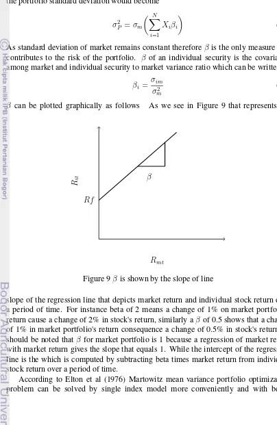
β can be plotted graphically as follows As we see in Figure 9 that represents the
Rit
Rmt
β
Rf
Figure 9βis shown by the slope of line
slope of the regression line that depicts market return and individual stock return over a period of time. For instance beta of 2 means a change of 1% on market portfolio's return cause a change of 2% in stock's return, similarly aβof 0.5 shows that a change of 1% in market portfolio's return consequence a change of 0.5% in stock's return. It should be noted thatβ for market portfolio is 1 because a regression of market return with market return gives the slope that equals 1. While the intercept of the regression line is the which is computed by subtracting beta times market return from individual stock return over a period of time.
accuracy. Kuhn Tucker conditions stated earlier can be satisfied by solving single index model to obtain optimized portfolio when short sales are disallowed. By modifying Equation (47) for single index model and substituting Zi as the value of
λXiwe get
Equation (53) is the first Kuhn Tucker condition which is made an equality by introducing variableUi . Second condition stated that the product of Zi andUi equal
zero. Third condition is about non-negativity of Zi and Ui such that when if Zi is
positive thenUiequals zero and vice versa. Above equation include securities that are
in the optimized portfolio and this optimal set is represented by k. Therefore any security for whichZj = 0are excluded. By settingU−iequal zero the above equation
become
And the value forC∗can be derived from Equation (53) which is
C∗ =
C∗ represent Cut Off rate, which indicates that any stock with excess return toβ ratio below the value of Cut Off rate would be excluded from the optimized portfolio assuming that single index model is an adequate measure of return structure and short sales are not allowed. We can write it as follows
¯
Ri−RF
β > C
∗ (58)
Optimal portfolio include all those stocks who have excess return to beta ratio higher than C∗. We can see the above results satisfied the Kuhn Tucker conditions. The second condition that product of theZiUi = 0 is met by construction as we putUi equals zero
andZipositive in Equation (54). We mentioned that only securities withZi >0would
be included in the optimal portfolio, here Ui = 0 and this satisfies the third Kuhn
Previous Researches
1. Pilotteet al.(2006) implemented single index"model using US Treasury bonds data from 1959-1997 where it was found that Sharpe ratios for short maturities are very high, for 3-month bills about 11 times the magnitude of Sharpe ratios on 5-year bonds. Sharpe ratios on long-term bonds are lower and, for maturities of more than a year, of a magnitude similar to those on common stocks".
2. Bilbao et al. (2007) proposed a "methodological extension of Sharpe's single index model, called Sharpe'model with expert Betas. This extension has been carried out through the construction of Betas obtained from both, statistical and imprecise expert estimations taking, also, into account several views of the market".
3. Caporin et al. (2013) "introduce a Conditional Single Index model where the time-varying alpha and beta parameters depend only on the past history of the underlying portfolio returns and of the benchmark returns".
4. Kwan (1995) "presented and formally justified a simple yet versatile ranking method for portfolio construction under institutional procedures for short selling".
5. Huang (2012) "discusses a multi-period portfolio selection problem when security returns are given by expert's evaluations".
6. Farinelli et al. (2008) "develop an integrated decision aid system for asset allocation based on a toolkit of eleven performance ratios".
7. Chenet al. (2009) "proposes a basic portfolio selection model in which future return rates and future risks of mutual funds are represented by triangular fuzzy numbers".
8. Fu et al. (2013) "adopted Genetic Algorithms to determine the optimized parameters setting of different technical indicators and portfolio weighting". 9. Bajeux-Besnainou et al. (2012) "introduce the Break-Down Free Generalized
Minimum Residual (BFGMRES), a Krylov subspaces method, as a fully automated approach for deriving the minimum variance portfolio".
10. Gokgozet al. (2012)"focuses on electricity generation asset allocation between bilateral contracts, such as forward contracts, and daily spot market, considering constraints of generating units and spot price risks. Mean-variance optimization has been successfully applied to all cases that modeled for electricity market". 11. Hjalmarsson et al. (2012) "study empirical mean-variance optimization when
the portfolio weights are restricted to be direct functions of underlying stock characteristics such as value and momentum".
12. Kawaset al. (2011)"extends the Log-robust portfolio management approach to the case with short sales, i.e., the case where the manager can sell shares he does not yet own".
in the primitive assets may not be possible".
14. Alexander et al. (2006) "find that while the constraint typically decreases the optimal portfolio's standard deviation, the constrained optimal portfolio can be notably mean-variance inefficient".
15. Choudhry et al. (2010) "empirically investigates the effects of the Asian financial crisis of 1997-98, and the period immediately afterwards, on the time-varying beta of four industrial sectors (chemical, finance, retail and industry) of Indonesia, Singapore, South Korea, and Taiwan. Results provide evidence of the influence of the Asian financial crisis, and the period after, on the time-varying industrial betas of these countries".
16. Chiou (2008) "suggest that local investors in the less developed countries, particularly in East Asia and Latin America, comparatively benefit more from both regional and global diversification".
17. Schwebach's (2002) "examination of the correlations and volatility of 11 foreign markets reveals that potential diversification benefits changed dramatically for the period following the devaluation of the baht by Thailand in July of 1997. Specifically, both the correlations and the volatilities increased substantially among the 11 countries following the July devaluation. This caused the efficient portfolio set to shift downward and to the right in the Markowitz mean-standard deviation space".
18. Bayuaji (2004) implemented single index model using data of LQ45 companies for the year 2003 in Indonesian stock market. This research computed optimal portfolio only and no further econometric treatment was conducted therefore it do not answer questions concerning portfolio diversification and parameter estimates.
19. Widyantini (2005) implemented single index model and constant correlation model using weekly data of LQ45 companies for the time period of 2003-2005 in Indonesian stock market. β value of portfolio is very close to marketβ both for single index model and constant correlation model. However he did not conduct any regression analysis of portfolios against market, therefore it can not be known that how much systematic risk is eliminated due to diversification. 20. Sumarna (2006) implemented single index model using monthly data of 30
securities for time period of 2005-2005 in Indonesian stock market. Portfolio β
is not very close to market β, however there are individual stocks with betas close to market.
21. Adisetya (2006) implemented both Markowitz and single index model using monthly data from 16 mutual funds for the time period of 2003-2006 in Indonesian stock market. He computed optimal portfolio comprising of all mutual funds, however systematic and unsystematic risk is computed only for individual mutual funds.
Research Framework
269 Stocks, Montlhy Stock Prices,
Indonesian Stock Market
Objectives
1. Analysis of Portfolio Optimization 2. Analysis of Portfolio Performance
Testing Assumptions of Linear Regression
1- Heteroskedasticity 2- Autocorrelation
⁀
Long and Short Portfolios
Method
Least Square Method
Model
Sharpe's Diagonal Model
Softwares
1- R 3.0.1 stockPortfolio package 2- EViews 6, 3- Treemap, 4- LaTex
Outcome
1-Optimized portfolio for all stocks at BEI with and without shortselling. 2-Performance evaluation of individual sector.
3-Contribution of each stock towards the market volatility.
Diagonal Model
Single index is the only common factor among varying stocks that covary with each other with reference to this common factor. For a single assetiit is (Zivot 2012).
Rit =αi+βRM t+εit (59)
whereRM t =Return on market index,
εit =Error term
Assumptions of the Diagonal model are as follows
cov(RM t, εit) = 0, cov(εit, εjt) = 0, cov(εit, εi,t−j) = 0 (60)
RM t ∽iid N(µM, σ
2
M), εit ∽iid N(0, σε,I2 ) (61)
αi, βi, µM, σ
2
M, σ
2
Statistical properties of the Diagonal model are
The study is an empirical and explanatory, and evidence are provided using data. Single index model is a linear regression model therefore it needs to satisfy following assumptions of classical linear regression model.
1. Mean value of error termuequals zero for any given value of Xi (Gujaratiet al.
2010).
E(u|Xi) = 0 (66)
2. Variance of each ui is homoscedastic, which means that given the values of
independent variable the values of independent variable around its mean values have same variance (Gujaratiet al. 2010).
var(ui) =σ
2
(67)
3. No autocorrelation between any two error terms (Gujaratiet al. 2010).
cov(ui, uj) = 0 (68)
Since there is no covariance among any two error terms and the value of independent variableY depends uponuthen
cov(Yi, Y j) = 0 (69)
4. The error termui is normally distributed with zero mean andσ
2
variance.
Ui ∽N(0, σ 2
) (70)
minSSR( ˆαi,βˆi) =
Once optimal portfolios are comuputed then we conducted performance analysis of these portfolios. Main three measures of performance are as follows:
1. Sharpe Measure: This measure is same as capital market line and also called asreward-to-variability ratio. It can be defined as the excess mean return over riskfree asset and ratio to total risk.
SharpeM easure= R¯p−Rf
σ(Rp)
(76)
Managers use this measure to evaluate whether excess return on portfolio can compensate higher risk involve in the portfolio when compare it with market portfolio. In case of well diversified portfolio, Sharpe measure reach close to market portfolio (Prigent 2007).
2. Treynor Measure: This measure is also known as reward-to-risk ratio. This ratio is similar to Sharpe ratio except that 'it uses systematic risk instead of total risk' (Bodieet al.2009).
T reynorM easure= R¯p−Rf
βp
(77)
3. Jensen Measure: This measure can be defined as portfolio return in excess to the return predicted by CAPM.
αp = (¯rp−rf)−βp( ¯RM −Rf) (78)
Jensen presented coefficientαp as performance measure, where managers seeks
portfolios with αp > 0. Furthermore a value of αp well above 0 prove
Research Limitations
It is assumed that stock prices incorporate all the available information therefore this research lack any form of qualitative data. The stock prices data are also collected from a short duration of five years which may not reflect the performance of stock prices in long run.
Data
Five years secondary data consisting of monthly stock prices are collected through IDX monthly statistics for all stocks listed at BEI during 2007-2011.
Table 3 Sectors Number of Stocks consistently Listed 2007-2011
No Name of Sector No of Stocks
1 Agriculture 8
2 Mining 8
3 Basic Industry and Chemicals 42
4 Miscellaneous Industry 32
5 Consumer Goods Industry 30
6 Property, Real Estate and Building Construction 26
7 Infrastructure, Utilities and Transportation 18
8 Finance 54
9 Trade, Services and Investment 51
Total 269
Portfolio Optimization with R
Markowitz portfolio theory has been implemented with various computing programs such as Benninga (2008) implemented it in Excel. One of the initial attempt was made by Sharpe (1963), when he used a programming code called RAND QP which was written in FORTRAN language and was run in IBM 7090. In this research R software (R Core Team 2012) is used to implement portfolio theory based on single index model. Here I will describe the R programming code used to compute the optimal portfolio. Stock prices are IDX monthly statistics and converted into .txt files. Data is read into R using read.table function. R code to read data is as follows
data<-read.table("stockprices.txt", header=TRUE)
Return on each stock is computed in R, for instance return for AALI is calculated by this R code
> AALI<-(data$AALI[-length(data$AALI)]-data$AALI[-1])/ data$AALI[-1]
After computing return for each individual stock as well as for market index, then we integrate all data using data.frame function which is as follows
stockreturns<-data.frame(AALI,UNSP,LSIP,MBAI,CPRO,DSFI,IIKP, BTEK,BUMI,PTBA,ENRG,MEDC,ANTM,INCO,TINS,CTTH,ARNA,
AMFG,IKAI,MLIA,TOTO,BUDI,SMCB,INTP,SMGR,ALMI,BTON, CTBN,INAI,JKSW,JPRS,LION,LMSH,PICO,TBMS,DPNS,EKAD, ETWA, SRSN,INCI,SOBI,AKKU,APLI,BRNA,IGAR,SIMA,FPNI, TRST,CPIN,JPFA,SIPD,SULI,TIRT,FASW,INKP,SAIP,SPMA,TKIM, ASII,AUTO,BRAM,GJTL,GDYR,IMAS, INDS,LPIN, MASA,NIPS, PRAS, SMSM, MYTX,ADMG,CNTX,ESTI, INDR,KARW,PBRX, PAFI,POLY, RICY,SSTM,TFCO,BATA,IKBI,JECC,KBLI,SCCO, VOKS,ERTX,HDTX,ADES,AISA,CEKA,DAVO,DLTA,INDF,MYOR, MLBI,PSDN,SKLT,STTP,ULTJ,MLBI,GGRM,HMSP, DVLA,SQBI,
KLBF,INAF,KAEF,MERK,PYFA,SCPI,TSPC,TCID,MRAT,UNVR, KICI,KDSI,LMPI,ELTY,BIPP,BKSL,CTRA,CTRS,DILD,DART,DUTI, FMII,GMTD,KPIG,KIJA,JPRT,LAMI,LPCK,LPKR,MDLN,PWON,
PWSI,RBMS,SIIP,SMDM,SMRA,ADHI,SSIA,TOTL, PGAS,CMNP,
BTEL, EXCL,ISAT,FREN,TLKM,APOL,BLTA,CMPP,HITS,IATA,MIRA, TMAS, RIGS,SMDR,SAFE, ZBRA,INPC,BABP,BBKP,BNBA,BBCA, BNGA,BBNP,BBRI,BDMN,BEKS,BNII,BKSW,BMRI,MEGA,BBNI,
BCIC,NISP,PNBN,BNLI,BVIC,SDRA,ADMF,BFIN, BBLD,CFIN,DEFI, INCF,MFIN, TRUS,WOMF,AKSI,HADE,KREN,PEGE,PANS,RELI,
MDRN, MICE,TGKA,UNTR,TURI,WAPO,WICO,ALFA,HERO, MPPA,MAPI,RALS,RIMO,SONA,BAYU,FAST,SHID,MAMI,PANR, PJAA,PTSP,PLIN,PNSE,PUDP,ABBA,FORU,IDKM,JTPE,SCMA, TMPO,ASGR,DNET,LMAS,MTDL,MLPL,BNBR, BMTR,PLAS,GEMA,
JKSE)
Once data.frame is created then date is removed and a matrix is constructed as follows:
> row.names(stockreturns) <- data$date[-60] > return.matrix <- as.matrix(stockreturns)
Optimal portfolio is computed using 'stockPortfolio 'package in R from Diez et al.
(2013). R code for short portfolio model is given below
modelshortSell<-stockModel(return.matrix,model="SIM", index=270)
Following is the R code for long portfolio model
> modelnoshortSell <- stockModel(return.matrix, model="SIM" ,index=270,shortSelling=’n’)
Finally optimal portfolios are constructed for both short and long portfolios
> OptimalPort.Short <- optimalPort(modelshortSell, Rf=0.00625, shortSell=NULL, eps = 10^(-4))
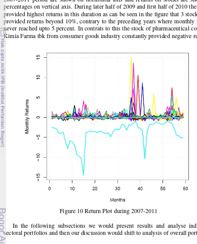
Monthly returns of all 269 stocks are plotted in Figure 10, where 60 months during 2007-2011 period are shown on horizontal axis and returns on stocks are shown in percentages on vertical axis. During later half of 2009 and first half of 2010 the stocks provided highest returns in this duration as can be seen in the figure that 3 stocks even provided returns beyond 10%, contrary to the preceding years where monthly returns never reached upto 5 percent. In contrats to this the stock of pharmaceutical company Kimia Farma tbk from consumer goods industry constantly provided negative return.
Figure 10 Return Plot during 2007-2011
In the following subsections we would present results and analyse individual sectoral portfolios and then our discussion would shift to analysis of overall portfolios.
Agriculture Sector
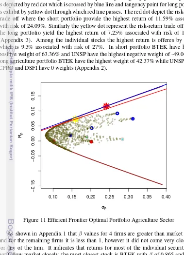
stocks with short and long restrictions respectively. Tangency point for short portfolio is depicted by red dot which is crossed by blue line and tangency point for long portfolio is exhibit by yellow dot through which red line passes. The red dot depict the risk-return trade off where the short portfolio provide the highest return of 11.59% associated with risk of 24.09%. Similarly the yellow dot represent the risk-return trade off where the long portfolio yield the highest return of 7.25% associated with risk of 15.89% (Appendix 3). Among the individual stocks the highest return is offeres by BTEK which is 9.3% associated with risk of 27%. In short portfolio BTEK have highest positive weight of 63.36% and UNSP have the highest negative weight of -49.06%. In long agriculture portfolio BTEK have the highest weight of 42.37% while UNSP, LSIP, CPRO and DSFI have 0 weights (Appendix 2).
0.10 0.15 0.20 0.25 0.30 0.35 0.40
−0.15
−0.05
0.00
0.05
0.10
0.15
σp
Rp ●
● ●
●
●
●
●
●
●
Figure 11 Efficient Frontier Optimal Portfolio Agriculture Sector
As shown in Appendix 1 that β values for 4 firms are greater than market β of 1 and for the remaining firms it is less than 1, however it did not come very close to 1 for any of the firm. It indicates that returns for most of the individual securities did not follow market closely, the most closest stock is BTEK withβ of 0.865 and AALI withβ of 1.23. Standard errors forβranges from 0.165 to 0.508 which are quite large for individual stocks. The assumption thatβ equal to 1 is tested and t-values for five individual stocks are found to be less than 2, therefore the hypothesis that theirβequals 1 can not be rejected. R2
of 30%. It can be infer from these values that variance in stock returns are not well explained by market return. In other words the low R2
indicates that most of the stock variance is firm specific and not related with market.
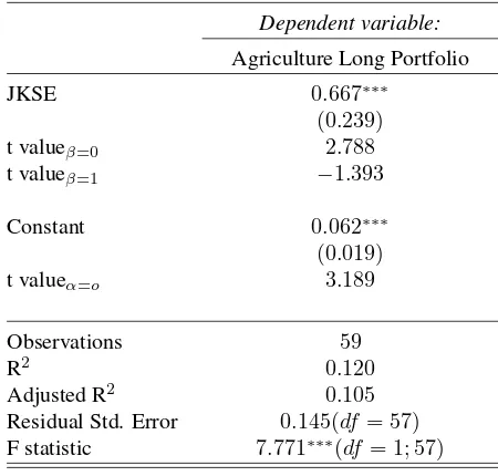
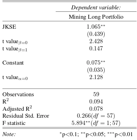
The optimal long portfolio include 4 firms which are AALI, MBAI, IIKP and BTEK. The β for this long portfolio is 0.667 as can be seen in Table 4 which is not very close to market β as there are 3 stocks having β closer to market. Portfolios should have aβ more closer to market β than any individual stock which constitute it but it did not happen in this case. Similarly theβ standard error for portfolioβ which is 0.239 is not the most accurate one in terms of estimation as the standard error of 0.179 for AALI β is lower. However the test of hypothesis that portfolio β equals 1 can not be rejected as t-value is less than 2.
Table 4 Regression Agriculture Long Portfolio against Market Return
Dependent variable:
Agriculture Long Portfolio
JKSE 0.667∗∗∗
(0.239)
t valueβ=0 2.788
t valueβ=1 −1.393
Constant 0.062∗∗∗
(0.019)
t valueα=o 3.189
Observations 59
R2
0.120
Adjusted R2
0.105
Residual Std. Error 0.145(df= 57)
F statistic 7.771∗∗∗(df = 1; 57)
Note: ∗p<0.1;∗∗p<0.05;∗∗∗p<0.01
The residual standard error also does not support the theory that adding more stocks in portfolio make residual error irrelevant due to diversification effect. This can be seen by comparing value of portfolio residual standard error with the values residual standard errors of individual stocks, where although the portfolio standard error of 0.145 is lower than many of stocks but it is not the lowest compare to AALI with 0.108. Similarly R2
represent the systematic risk and 1- R2
represent the unsystematic risk. A portfolio should have a larger systematic risk than individual stocks due to diversification effect. Portfolio R2
is 12% which is lower than the values of most individual stocks R2
. It can be infer that market variance do not explain most of the portfolio variance.
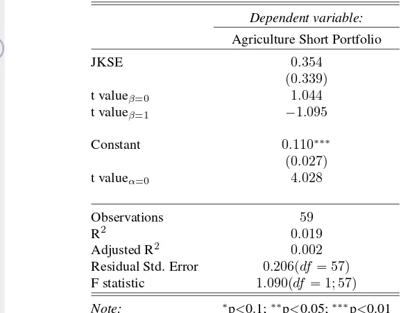
stocks are included in the portfolio. The short portfolioβis 0.354 as shown in Table 5 which lies far away from the marketβ.
Table 5 Regression Agriculture Short Portfolio against Market Return
Dependent variable:
Agriculture Short Portfolio
JKSE 0.354
(0.339)
t valueβ=0 1.044
t valueβ=1 −1.095
Constant 0.110∗∗∗
(0.027)
t valueα=0 4.028
Observations 59
R2
0.019
Adjusted R2
0.002
Residual Std. Error 0.206(df = 57)
F statistic 1.090(df = 1; 57)
Note: ∗p<0.1;∗∗p<0.05;∗∗∗p<0.01
Test of hypothesis that agriculture short portfolioβ equals 1 can not be rejected as its t-value is less than 2. Similarly the residual standard error of 0.206 is larger than any individual stock which shows that error term is not irrelevant and diversification effect is not found despite of including all stocks from agriculture sector in this portfolio. The value of R2
for short portfolio is extremely low that is 1.9%, which means a tiny proportion of agriculture short portfolio variance is explained by market variance. These empirical evidence do not support the theory of diagonal model.
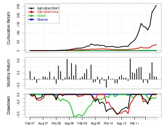
Performance of long and short portfolios as well as return provided by market index and risk free rate are illustrated by Figure 12. This figure display cumulative return, monthly return and drawdown where returns are on y-axis and monthly time period is on x-axis. Cumulative return reached beyond 25000% for agriculture short portfolio and outperformed agriculture long portfolio which provided cumulative return close to 4000%. Monthly returns chart shows that most of the monthly returns are positive. Finally from the drawdown chart it can seen that long and short portfolios followed each other and they dropped down during the mid of 2009 till the mid of 2010 when they started going up. Contrary to this market index got down during fall of 2008 when financial crisis hit the US stock market and it went up during first quarter of 2009.
0
50
100
150
200
250 ● AgricultureShort
AgricultureLong
Market
Riskfree
Cum
ulativ
e Retur
n
−0.2
0.2
0.6
Monthly Retur
n
Feb 07 Aug 07 Feb 08 Aug 08 Feb 09 Aug 09 Feb 10 Aug 10 Feb 11
Date
−0.5
−0.2
0.0
Dr
a
wdo
wn
Figure 12 Performance Chart Agriculture Portfolio
short portfolio is higher than 42% from agriculture long portfolio, however with larger volatility. Investor should favor agriculture short portfolio due to higher Sharpe ratio. Similar results are obtained for Treynor ratio where only systematic risk is accounted rather than total risk. Finally the positive values of α obtained from Jensen measure indicate that both agriculture short and long optimal portfolios outperformed the market. However 11% Jensen ratio for agriculture short portfolio is larger than 6% for agriculture long portfolio, depicting that former beat the market with greater margin than later.
Mining Sector Portfolio
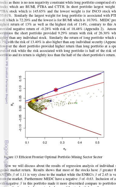
stocks as there is no non negativity constraint while long portfolio comprised of only 3 stocks which are BUMI, PTBA and CTTH. In short portfolio largest weight is for PTBA stock which is 145.65% and the lowest weight is for INCO stock which is -55.61%. Similarly the largest weight for long portfolio is associated with PTBA as well which is 72.20% and the lowest is for BUMI which is 10.70%. MEDC provided highest return of 13% as well as the highest risk of 114%, contrary to this ANTM provided negative return of -0.28% with risk of 18.48% (Appendix 2). Among two portfolios the short portfolio provided 9.29% return with risk of 26.30% which is higher than any individual stock. Similarly the return of long portfolio which equals 3.7% with the risk of 13.40% is also higher than any individual security (Appendix 3). However the short portfolio provided higher return than long portfolio at a specified level of risk while the risk associated with long portfolio is half of the risk of short portfolio and its return is slightly less than the half of the short portfolio's return.
0.1 0.2 0.3 0.4 0.5
−0.10
−0.05
0.00
0.05
0.10
0.15
σp Rp
●
●
●
●●●
●
●
Figure 13 Efficient Frontier Optimal Portfolio Mining Sector Sector