Organisasi Komputer (T. Informatika)

(1)

Appendix B: Reduction of Digital Logic B-1

Principles of Computer Architecture

Miles Murdocca and Vincent Heuring

(2)

Appendix B: Reduction of Digital Logic B-2

Chapter Contents

B.1 Reduction of Combinational Logic and Sequential Logic B.2 Reduction of Two-Level Expressions

(3)

Appendix B: Reduction of Digital Logic B-3

Reduction (Simplification) of Boolean

Expressions

• It is usually possible to simplify the canonical SOP (or POS) forms.

• A smaller Boolean equation generally translates to a lower gate count in the target circuit.

(4)

Reduced Majority Function Circuit

• Compared with the AND-OR circuit for the unreduced majority

function, the inverter for C has been eliminated, one AND gate has been eliminated, and one AND gate has only two inputs instead of three inputs. Can the function by reduced further? How do we go about it?

F

A B C

F

A B C

A B C

Unreduced

(5)

The Algebraic Method

• Consider the majority function, F. We apply the algebraic method to reduce F to its minimal two-level form:

F ABC AB C ABC ABC

F ABC AB C AB C C

F ABC AB C AB

F ABC AB C AB ABC

F ABC AC B B AB

F ABC AC AB

F ABC AC AB ABC

F BC

= + + +

= + +

= + + +

= + +

= + + +

=

( )

Distributive Property Complement Property Identity Property

Idempotence Identity Property Complement and Identity

Idempotence 1

((A A) AC AB

F BC AC AB

+ + +

= + +

Distributive

(6)

The Algebraic Method

• This majority circuit is functionally equivalent to the previous ma-jority circuit, but this one is in its minimal two-level form:

F

(7)

Karnaugh Maps: Venn Diagram

Rep-resentation of Majority Function

• Each distinct region in the “Universe” represents a minterm.

• This diagram can be transformed into a Karnaugh Map.

ABC

ABC’ _AB’C’ _AB’C

A’BC

A’BC’ A’B’C

A’B’C’ B

A

(8)

K-Map for Majority Function

• Place a “1” in each cell that corresponds to that minterm.

• Cells on the outer edge of the map “wrap around”

A B C F

Minterm Index

0 0 0 0

0 0 1 0

0 1 0 0

0 1 1 1

1 0 0 0

1 0 1 1

1 1 0 1

1 1 1 1

0 1 2 3 4 5 6 7

1 0

0-side 1-side 0

A balance tips to the left or right depending on whether

there are more 0’s or 1’s.

00

01

11

10

0

1

AB

C

1

(9)

Adjacency Groupings for Majority

Function

• F = BC + AC + AB

00

01

11

10

0

1

AB

C

1

(10)

Appendix B: Reduction of Digital Logic B-10

Minimized AND-OR Majority Circuit

• F = BC + AC + AB

• The K-map approach yields the same minimal two-level form as

F

(11)

K-Map Groupings

• Minimal grouping is on the left, non-minimal (but logically equiva-lent) grouping is on the right.

• To obtain minimal grouping, create smallest groups first.

00 01 11

1 01 11 1 1 10 AB 1 CD 10 00 01 11 01 11 10 CD 10 00 00 AB 1 1 1 1 1 2 3 4 1 1 1 1 1 1 1 1 2 4 5 1

F = A B C + A C D + A B C + A C D

F = B D + A B C + A C D + A B C + A C D

(12)

K-Map Corners are Logically Adjacent

00 01 11

1

1 01

11

1

1 1

10

AB

1

CD

00

(13)

Appendix B: Reduction of Digital Logic B-13

K-Maps and Don’t Cares

• There can be more than one minimal grouping, as a result of don’t cares.

00 01 11

1 01

11

1 1

10

AB

1

CD

10 d

00 d

F = B C D + B D

01 11

1 01

11

1 1

10 1

CD

10 d

00 d

00

AB

F = A B D + B D

(14)

Five-Variable K-Map

• Visualize two 4-variable K-maps stacked one on top of the other; groupings are made in three dimensional cubes.

01 11

001 011

10

CDE

010 000

00

AB

01 11

101 111

10

CDE

110 100

00

AB

1 1

(15)

Six-Variable K-Map

• Visualize four 4-variable K-maps stacked one on top of the other; groupings are made in three dimensional cubes.

001 011

010

DEF

010 000

000

ABC

001 011

101 111

010

DEF

110 100

000

ABC

101 111

001 011

110

DEF

010 000

100

ABC

101 111

110

DEF

110 100

100

ABC

1

1 1

1

1 1

1

(16)

3-Level Majority Circuit

• K-Kap Reduction results in a reduced two-level circuit (that is, AND followed by OR. Inverters are not included in the two-level count). Algebraic reduction can result in multi-level circuits with even fewer logic gates and fewer inputs to the logic gates.

M

(17)

Map-Entered Variables

• An example of a K-map with a map-entered variable D.

00 01 11 10

0

1

AB C

1 1

D

(18)

Appendix B: Reduction of Digital Logic B-18

Two Map-Entered Variables

• A K-map with two map-entered variables D and E.

• F = BC + ACD + BE + ABCE

00 01 11 10

0

1

AB C

1 1

(19)

Appendix B: Reduction of Digital Logic B-19

Truth Table with Don’t Cares

(20)

Appendix B: Reduction of Digital Logic B-20

Tabular (Quine-McCluskey) Reduction

• Tabular reduction

be-gins by grouping

minterms for which F is nonzero according to the number of 1’s in each minterm. Don’t cares are considered to be nonzero.

• The next step forms a consensus (the logical form of a cross prod-uct) between each pair of adjacent groups for all terms that differ in

0 0 1 0 1 1 1 1 0 1 0 1 1 1 0 0 1 1 1 1 C D 0 0 0 1 1 0 1 0 1 1 B 0 0 0 0 0 1 0 1 1 1 A √ √ √ √ √ √ √ √ √ √ 0 _ 0 1 1 _ 0 1 1 1 1 _ _ 1 1 1 1 1 1 _ _ 1 1 1 C D 0 0 _ _ 0 1 1 1 0 1 _ 1 B 0 0 0 0 _ 0 _ 0 1 _ 1 1 A * √ √ √ √ √ √ * * √ √ √ _ 1 _ 1 1 1 C D _ _ 1 B 0 _ _ A * * * Initial setup After first

reduction After secondreduction

(a)

(b)

(21)

Appendix B: Reduction of Digital Logic B-21

Table of Choice

• The prime implicants form a set that completely covers the func-tion, although not necessarily minimally.

• A table of choice is used to obtain a minimal cover set.

0

1

0

_

_ 0

1

0

_

1 0

1

_

1

_ _

_

1

0001 0011 0101 0110 0111 1010 1101 Minterms

Prime Implicants

√

√ √

√ √ √ √

√ √

√ √ √

*

(22)

Reduced Table of Choice

• In a reduced table of choice, the essential prime implicants and the minterms they cover are removed, producing the eligible set. • F = ABC + ABC + BD + AD

0

_

0

_

0

_

1

_

1

0001 0011

Minterms

Eligible

Set

√

Set 1

0 0 0 _

_ _ 1 1

Set 2

0 _ _ 1

X

Y

Z

√

(23)

Appendix B: Reduction of Digital Logic B-23

Multiple Output Truth Table

• The power of tabular reduction comes into play for multiple func-tions, in which minterms can be shared among the functions.

(24)

Multiple Output Table of Choice

F₀(A,B,C) = ABC + BC

F₁(A,B,C) = AC + AC + BC

F₂(A,B,C) = B

0

1

_

1 0

_

1

1 0

1

0

_

_ Prime

Implicants

√

m₀m₃m₇ m₁m₃m₄m₆m₇ m₂m₃m₆m₇ F₀(A,B,C) F₁(A,B,C) F₂(A,B,C)

Min-terms

F₀ F₁ F₁ F₂ F_1,2

√ √

√ √ √ √

√ √

*

(25)

Appendix B: Reduction of Digital Logic B-25

Speed and Performance

• The speed of a digital system is governed by: • the propagation delay through the logic gates and • the propagation delay across interconnections.

(26)

Propagation Delay for a NOT Gate

• (From Hamacher et. al. 1990)

+5V

0V

+5V

0V

10%

90% Transition Time

90%

10% 50%

(2.5V)

50% (2.5V) Propagation Delay

Transition Time A NOT gate

input changes from 1 to 0

The NOT gate output changes from 0 to 1

(Fall Time)

(Latency)

(27)

Appendix B: Reduction of Digital Logic B-27

MUX Decomposition

A C F 0000 0001 0010 0011 B 0100 0101 0110 0111 1000 1001 1010 1011 1100 1101 1110 1111 D 1 0 0 1 0 1 1 0 0 1 0 0 0 0 0

1 _{A D}

F 00 01 10 11 B C 00 01 10 11 B C 00 01 10 11 1 0 0 1 0 1 1 0 0 B C+ B C

B C + B C

F ABCD AB C D AB CD ABC D ABCD AB C D ABCD B C BC AD B C BC AD B C BC

( )

( ) ( ) ( )

= + + + + +

(28)

OR-Gate Decomposition

• Fanin affects circuit depth.

A + B + C + D A BCD

Associative law of Boolean algebra: Initial high fan-in gate

Balanced tree

A B CD

(A + B) + (C + D)

(29)

State Reduction

• Description of state machine M0 to be reduced.

X

0

1

A

C/0

E/1

Present state

Input

B

C

D

E

D/0

E/1

C/1

B/0

C/1

A/0

(30)

Appendix B: Reduction of Digital Logic B-30

Distinguishing Tree

• A next state tree for M0.

(ABCDE)

(CDA)(CC)

(ABE)(CD)

(CC)(C)(CC)

(AB)(E)(CD)*

(BA)(E)(BB)

(AB)(E)(CD)

(DC)(A)(DD)

(AB)(E)(CD)

(EE)(C)(EE)

(AB)(E)(CD)*

(CC)(C)(CC) (AB)(E)(AA)

(AB)(E)(CD)

(EEC)(BA)

(ABE)(CD)

(AA)(C)(DC)

(AB)(E)(CD)

(CC)(B)(EE)

(AB)(E)(CD)*

(CC)(C)(CC) (EE)(B)(AB)

0 1

Next states

(31)

Reduced State Table

• A reduced state table for machine M1.

X

0

1

AB: A'

B'

/0

C'

/1

Current state

Input

CD: B'

E: C'

B'

/1

A'

/0

(32)

Appendix B: Reduction of Digital Logic B-32

The State Assignment Problem

• Two state assignments for machine M2.

P.S.

Input X

0 1

A B/1 A/1

B C/0 D/1

C C/0 D/0

D B/1 A/0

Machine M₂

Input X

0 1

A: 00 01/1 00/1 B: 01 10/0 11/1 C: 10 10/0 11/0 D: 11 01/1 00/0

State assignment SA₀

S₀S₁

Input X

0 1

A: 00 01/1 00/1 B: 01 11/0 10/1 C: 11 11/0 10/0 D: 10 01/1 00/0

State assignment SA₁

(33)

State Assignment SA

₀

• Boolean equations for machine M2 using state assignment SA0.

01

11

1

10

X

0 00

S₀S₁

1 1

01

11

1

10 0 00 1

1

1 1

X S₀S₁

01

11

1

10 0

00 ₁ ₁

1

X S₀S₁

S₀ = S₀S₁ + S₀S₁ Z = S₀S₁ + S₀X

+ S₀S₁X S₁ = S₀S₁X + S₀S₁X

(34)

State Assignment SA

1

• Boolean equations for machine M2 using state assignment SA1.

01

11

1

10

X

0 00

S₀S₁

1 1

01

11

1

10 0 00 1

1

1 1

X

S₀S₁

01

11

1

10 00

X

1 1

1

S₀S₁ 0

S₁ = X

(35)

Sequence Detector State Transition

Diagram

A

B

0/0

1/0

C

D

E

F

G

0/0

1/0

0/0

1/0

0/0

1/0 1/0

1/1 0/0

1/1

0/0

0/1 Input: 0 1 1 0 1 1 1 0 0

(36)

Appendix B: Reduction of Digital Logic B-36

Sequence Detector State Table

X

0 1

A B/0 C/0

Present state Input

B C D E

D/0 E/0 F/0 G/0 D/0 E/0 F/0 G/1

F D/0 E/1

(37)

Appendix B: Reduction of Digital Logic B-37

Sequence Detector Reduced State

Table

X

0

1

B'

/0

C'

/0

Present state

Input

B'

/0

D'

/0

E'

/0

F'

/0

E'

/0

F'

/1

B'

/0

D'

/1

E'

/1

F'

/0

(38)

Appendix B: Reduction of Digital Logic B-38

Sequence Detector State Assignment

X

0 1

A': 000 001/0 010/0

Present state

Input

B': 001 C': 010 D': 011 E': 100

001/0 011/0 100/0 101/0 100/0 101/1 001/0 011/1

F': 101 100/1 101/0

(39)

Appendix B: Reduction of Digital Logic B-39

Excitation Tables

• In addition to the D flip-flop, the S-R, J-K, and T flip-flops are used as delay elements in finite state machines.

• A Master-Slave J-K flip-flop is shown below.

Q Q J

CLK

J

Q Q

K

Circuit Symbol

(40)

Sequence Detector K-Maps

• K-map re-duction of next state and output functions for sequence detector. 01 11 10 00

S₀X

1 1 1 1

01 11 10

d d d d 1 1 1 1 00

S₂S₁

01 11 10 00

S₀X

1 1

01 11 10

d d d d 1 00

S₂S₁

01 11 10 00

S₀X

1 10 d d d 00

S₂S₁

01 11 10 00

S₀X 01 11 10

d d d 1 1 00

S₂S₁

01 11

S₀ = S₂S₁X +S₀X

+S₂S₀ +S₁X

S₁ = S₂S₁X +S₂S₀X

1 1

(41)

Appendix B: Reduction of Digital Logic B-41

Clocked T Flip-Flop

• Logic diagram and symbol for a T flip-flop.

J

Q Q

K

Circuit

Q Q

Symbol 1

(42)

Appendix B: Reduction of Digital Logic B-42

Sequence

Detector

Circuit

CLK

Q D

Q S₀

Q D

Q S₁

Q D

(43)

Appendix B: Reduction of Digital Logic B-43

Excitation Tables

• Each table

shows the set-tings that must be applied at the inputs at time t in order to

change the out-puts at time t+1.

0 0 1 1 0 1 0 1

Q_t Q_t+1 _S

0 1 0 0 R 0 0 1 0 S-R flip-flop 0 0 1 1 0 1 0 1

Q_t Q_t+1 _D

0 1 0 1 D flip-flop 0 0 1 1 0 1 0 1

Q_t Q_t+1 _J

0 1 d d K d d 1 0 J-K flip-flop 0 0 1 1 0 1 0 1

Q_t Q_t+1 _T

(44)

Serial Adder

Serial Adder 0 1 1 0 0

0 1 1 1 0

1 1 0 1 0

X Y

Z C_in C_out

4 3 2 1 0

4 3 2 1 0 Time (t)

Time (t)

A B

00/0 01/1

10/1

11/0

00/1

10/0 01/0

11/1 No carry

state Carry state

x_i y_i

z_i

Present state (S_t)

Input XY

00 01 10 11

Present state

Input XY

00 01 10 11

A A/0 A/1 A/1 B/0

B A/1 B/0 B/0 B/1

Next state Output

(45)

Appendix B: Reduction of Digital Logic B-45

Serial Adder Next-State Functions

• Truth table showing next-state functions for a serial adder for D,

S-R, T, and J-K flip-flops. Shaded functions are used in the ex-ample. 0 0 1 1 0 0 1 1 0 1 0 1 0 1 0 1

Y S_t

0 0 0 0 1 1 1 1 X 0 0 0 1 0 1 1 1 D 0 0 0 0 0 0 1 0 S 0 1 0 0 0 0 0 0 R 0 d 0 d 0 d 1 d J d 1 d 0 d 0 d 0 K 0 1 0 0 0 0 1 0 T 0 1 1 0 1 0 0 1 Z Present

(46)

Appendix B: Reduction of Digital Logic B-46

J-K Flip-Flop Serial Adder Circuit

CLK

Q J X

Y

Q

X Y

Y

X

Z S K X

(47)

Appendix B: Reduction of Digital Logic B-47

D Flip-Flop Serial Adder Circuit

CLK

Q D X

Y

Q

X Y

Y

X

Z S X

(48)

Appendix B: Reduction of Digital Logic B-48

Majority Finite State Machine

A

0/0

B

C

D

E

F

G

0/1

1/0

0/0

1/0

0/0

1/0

0/0

1/0

0/0 1/1

0/0 _1/1

Input: 0 1 1 1 0 0 1 0 1 Output: 0 0 1 0 0 0 0 0 1 Time: 0 1 2 3 4 5 6 7 8 Input History _ _ _

0 _ _

1 _ _

0 0 _ 0 1 _

(49)

Appendix B: Reduction of Digital Logic B-49

Majority FSM State Table

• (a) State table for majority FSM; (b) partitioning; (c) reduced state table.

X

0 1

A B/0 C/0

P.S. Input

B C D E

D/0 E/0 F/0 G/0 A/0 A/0 A/0 A/1 F A/0 A/1 G A/1 A/1

(a)

X

0 1

B'/0 C'/0 D'/0 E'/0 E'/0 F'/0 A'/0 A'/0 A'/0 A'/1 A'/1 A'/

1

A: A' B: B' C: C' D: D' EF: E'

G: F'

(c)

P₀ = (ABCDEFG) P₁ = (ABCD)(EF)(G) P₂ = (AD)(B)(C)(EF)(G) P₃ = (A)(B)(C)(D)(EF)(G) P₄ = (A)(B)(C)(D)(EF)(G) √

P.S. Input

(50)

Majority FSM State Assignment

• (a) State assignment for reduced majority FSM using D flip-flops; and (b) using T flip-flops.

X

0 1

A': 000 001/0 010/0

P.S.

Input

B': 001 C': 010 D': 011 E': 100

011/0 100/0 100/0 101/0 000/0 000/0 000/0 000/1

F': 101 000/1 000/1 S₂S₁S₀ S₂S₁S₀Z S₂S₁S₀Z

X

0 1

A': 000 001/0 010/0

P.S.

Input

B': 001 C': 010 D': 011 E': 100

000/0 010/0 110/0 111/0 011/0 011/0 100/0 100/1

F': 101 101/1 101/1 S₂S₁S₀ T₂T₁T₀Z T₂T₁T₀Z

(51)

Majority FSM Circuit

(52)

Chapter 1: Introduction 1-1

Principles of Computer Architecture

(53)

Chapter 1: Introduction 1-2

Chapter Contents

1.1 Overview

1.2 A Brief History

1.3 The Von Neumann Model 1.4 The System Bus Model 1.5 Levels of Machines

1.6 Upward Compatibility 1.7 The Levels

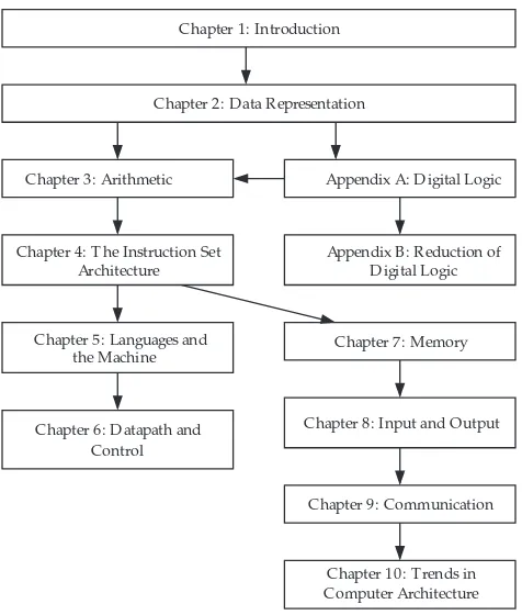
1.8 A Typical Computer System 1.9 Organization of the Book

(54)

Chapter 1: Introduction 1-3

Some Definitions

• Computer architecture deals with the functional behavior of a

computer system as viewed by a programmer (like the size of a data type – 32 bits to an integer).

• Computer organization deals with structural relationships that are

not visible to the programmer (like clock frequency or the size of the physical memory).

• There is a concept of levels in computer architecture. The basic idea is that there are many levels at which a computer can be con-sidered, from the highest level, where the user is running

(55)

Chapter 1: Introduction 1-4

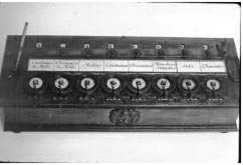
Pascal’s Calculating Machine

• Performs basic arithmetic operations (early to mid 1600’s). Does not have what may be considered the basic parts of a computer. • It would not be until the 1800’s until Babbage put the concepts of

mechanical control and mechanical calculation together into a machine that has the basic parts of a digital computer.

(56)

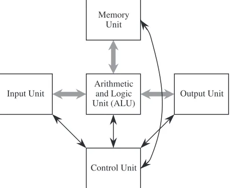
Input Unit Arithmetic and Logic

Unit (ALU) Output Unit Memory

Unit

Control Unit

The von Neumann Model

• The von Neumann model consists of five major components:

(57)

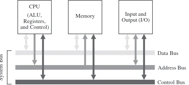
System Bus

Data Bus

Address Bus

Control Bus (ALU,

Registers, and Control)

Memory Input and Output (I/O) CPU

The System Bus Model

• A refinement of the von Neumann model, the system bus model has a CPU (ALU and control), memory, and an input/output unit. • Communication among components is handled by a shared

(58)

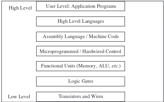
High Level

High Level Languages User Level: Application Programs

Functional Units (Memory, ALU, etc.)

Logic Gates

Assembly Language / Machine Code

Microprogrammed / Hardwired Control

Levels of Machines

• There are a number of levels in a computer (the exact number is open to debate), from the user level down to the transistor level. • Progressing from the top level downward, the levels become less

(59)

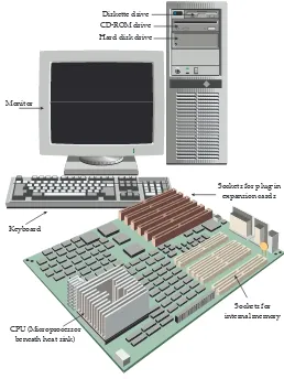
Monitor

CD-ROM drive Hard disk drive

Keyboard

Sockets for internal memory CPU (Microprocessor

beneath heat sink)

Sockets for plug-in expansion cards Diskette drive

(60)

Memory

Input / output

Battery Plug-in expansion card slots

Power supply connector Pentium II processor slot

(ALU/control)

The Motherboard

• The five von Neumann components are visible in this example motherboard, in the context of the system bus model.

(61)

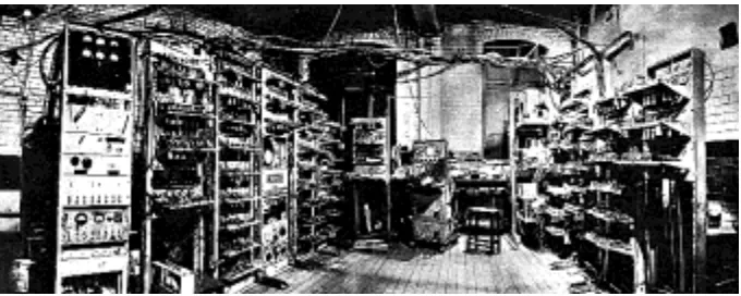
Manchester University Mark I

• Supercomputers, which are produced in low volume and have a high price, have been largely displaced by, high-volume low-priced machines that offer a better price-to-performance ratio.

(62)

Moore’s Law

• Computing power doubles every 18 months for the same price. • Project planning needs to take this observation seriously: an

(63)

Chapter 2: Data Representation 2-1

Principles of Computer Architecture

(64)

Chapter 2: Data Representation 2-2

Chapter Contents

2.1 Introduction

2.2 Fixed Point Numbers 2.3 Floating Point Numbers

2.4 Case Study: Patriot Missile Defense Failure Caused by Loss of Precision

(65)

Fixed Point Numbers

• Using only two digits of precision for signed base 10 numbers, the range (interval between lowest and highest numbers) is

[-99, +99] and the precision (distance between successive num-bers) is 1.

• The maximum error, which is the difference between the value of a real number and the closest representable number, is 1/2 the

pre-cision. For this case, the error is 1/2 × 1 = 0.5.

(66)

Weighted Position Code

• The base, or radix of a number system defines the range of pos-sible values that a digit may have: 0 – 9 for decimal; 0,1 for binary. • The general form for determining the decimal value of a number is

given by:

Example:

541.25₁₀ = 5 × 102 + 4 × 101 + 1 × 100 + 2 × 10-1 + 5 × 10-2

(67)

Base Conversion with the Remainder

Method

• Example: Convert 23.37510 to base 2. Start by converting the

inte-ger portion:

23/2 = 11 R 1 11/2 = 5 R 1 5/2 = 2 R 1 2/2 = 1 R 0 1/2 = 0 R 1

Integer Remainder

Least significant bit

(68)

Base Conversion with the

Multiplica-tion Method

• Now, convert the fraction:

.375 × 2 = 0.75

.75 × 2 = 1.50

.5 × 2 = 1.00

Least significant bit Most significant bit

(69)

Nonterminating Base 2 Fraction

• We can’t always convert a terminating base 10 fraction into an

equivalent terminating base 2 fraction:

.2

.4

.8

.6

.2

. . .

0.4

0.8

1.6

1.2

0.4 =

=

= 2

2

×

(70)

Base 2, 8, 10, 16 Number Systems

• Example: Show a column for ternary (base 3). As an extension of

that, convert 14 to base 3, using 3 as the divisor for the

(71)

More on Base Conversions

• Converting among power-of-2 bases is particularly simple:

1011₂ = (10₂)(11₂) = 23₄

23₄ = (2₄)(3₄) = (10₂)(11₂) = 1011₂

101010₂ = (101₂)(010₂) = 52₈

01101101₂ = (0110₂)(1101₂) = 6D₁₆

• How many bits should be used for each base 4, 8, etc., digit? For

base 2, in which 2 = 21, the exponent is 1 and so one bit is used

for each base 2 digit. For base 4, in which 4 = 22, the exponent is

2, so so two bits are used for each base 4 digit. Likewise, for base

8 and base 16, 8 = 23 and 16 = 24, and so 3 bits and 4 bits are used

(72)

Binary Addition

• This simple binary addition example provides background for the signed number representations to follow.

Operands 0 0 + 0 0 Sum Carry out

Carry in ₀

0 1 + 1 0 0 1 0 + 1 0 0 1 1 + 0 1 0 Example: Carry

Addend: A

Augend: B

0 1 1 1 1 1 0 0 0 1 0 1 1 0 1 0 1 1 1 1 0 0 0 0

(73)

Signed Fixed Point Numbers

• For an 8-bit number, there are 28 = 256 possible bit patterns.

These bit patterns can represent negative numbers if we choose to assign bit patterns to numbers in this way. We can assign half of the bit patterns to negative numbers and half of the bit patterns to positive numbers.

• Four signed representations we will cover are: Signed Magnitude

(74)

Signed Magnitude

• Also know as “sign and magnitude,” the leftmost bit is the sign (0 = positive, 1 = negative) and the remaining bits are the magnitude.

• Example:

+25₁₀ = 00011001₂

-25₁₀ = 10011001₂

• Two representations for zero: +0 = 00000000₂, -0 = 10000000₂.

• Largest number is +127, smallest number is -127₁₀, using an 8-bit

(75)

One’s Complement

• The leftmost bit is the sign (0 = positive, 1 = negative). Negative of a number is obtained by subtracting each bit from 2 (essentially, complementing each bit from 0 to 1 or from 1 to 0). This goes both ways: converting positive numbers to negative numbers, and con-verting negative numbers to positive numbers.

• Example:

+25₁₀ = 00011001₂

-25₁₀ = 11100110₂

• Two representations for zero: +0 = 00000000₂, -0 = 11111111₂.

• Largest number is +127₁₀, smallest number is -127₁₀, using an

(76)

Two’s Complement

• The leftmost bit is the sign (0 = positive, 1 = negative). Negative of a number is obtained by adding 1 to the one’s complement tive. This goes both ways, converting between positive and nega-tive numbers.

• Example (recall that -25₁₀ in one’s complement is 11100110₂):

+25₁₀ = 00011001₂

-25₁₀ = 11100111₂

• One representation for zero: +0 = 00000000₂, -0 = 00000000₂.

(77)

Excess (Biased)

• The leftmost bit is the sign (usually 1 = positive, 0 = negative). Positive and negative representations of a number are obtained by adding a bias to the two’s complement representation. This goes both ways, converting between positive and negative num-bers. The effect is that numerically smaller numbers have smaller bit patterns, simplifying comparisons for floating point exponents.

• Example (excess 128 “adds” 128 to the two’s complement ver-sion, ignoring any carry out of the most significant bit) :

+12₁₀ = 10001100₂

-12₁₀ = 01110100₂

• One representation for zero: +0 = 10000000₂, -0 = 10000000₂.

(78)

BCD Representations in Nine’s and

Ten’s Complement

• Each binary coded decimal digit is composed of 4 bits.

0 0 0 0 (0)₁₀

0 0 1 1 (3)₁₀

0 0 0 0 (0)₁₀

0 0 0 1 (1)₁₀

(+301)₁₀

1 0 0 1 (9)₁₀

0 1 1 0 (6)₁₀

1 0 0 1 (9)₁₀

1 0 0 0 (8)₁₀

(–301)₁₀

1 0 0 1 (9)₁₀

0 1 1 0 (6)₁₀

1 0 0 1 (9)₁₀

(–301)₁₀

Nine’s complement

Ten’s complement Nine’s and ten’s complement (a)

(b)

(c)

• Example: Represent +079₁₀ in BCD: 0000 0111 1001

• Example: Represent -079₁₀ in BCD: 1001 0010 0001. This is

(79)

(80)

Base 10 Floating Point Numbers

• Floating point numbers allow very large and very small numbers to be represented using only a few digits, at the expense of preci-sion. The precision is primarily determined by the number of dig-its in the fraction (or significand, which has integer and fractional parts), and the range is primarily determined by the number of digits in the exponent.

• Example (+6.023 × 1023):

+

Sign

2 3 6 0 2

Exponent

(two digits) _{(four digits)}Significand Position of decimal point

(81)

Normalization

• The base 10 number 254 can be represented in floating point form

as 254 × 100, or equivalently as:

25.4 × 101, or 2.54 × 102, or .254 × 103, or .0254 × 104, or

infinitely many other ways, which creates problems when making comparisons, with so many representations of the same number. • Floating point numbers are usually normalized, in which the radix

(82)

Floating Point Example

• Represent .254 × 103 in a normalized base 8 floating point format

with a sign bit, followed by a 3-bit excess 4 exponent, followed by four base 8 digits.

• Step #1: Convert to the target base.

.254 × 103 = 254₁₀. Using the remainder method, we find that 254₁₀

= 376 × 80:

254/8 = 31 R 6 31/8 = 3 R 7 3/8 = 0 R 3

• Step #2: Normalize: 376 × 80 = .376 × 83.

(83)

Error, Range, and Precision

• In the previous example, we have the base b = 8, the number of significant digits (not bits!) in the fraction s = 4, the largest expo-nent value (not bit pattern) M = 3, and the smallest expoexpo-nent value m = -4.

• In the previous example, there is no explicit representation of 0, but there needs to be a special bit pattern reserved for 0 other-wise there would be no way to represent 0 without violating the normalization rule. We will assume a bit pattern of

0 000 000 000 000 000 represents 0.

(84)

Error, Range, and Precision (cont’)

• Largest representable number: bM × (1 - b-s) = 83 × (1 - 8-4)

• Smallest representable number: bm × b-1 = 8-4 - 1 = 8-5

• Largest gap: bM × b-s = 83 - 4 = 8-1

(85)

Error, Range, and Precision (cont’)

• Number of representable numbers: There are 5 components: (A) sign bit; for each number except 0 for this case, there is both a positive and negative version; (B) (M - m) + 1 exponents; (C) b - 1 values for the first digit (0 is disallowed for the first normalized

digit); (D) bs-1 values for each of the s-1 remaining digits, plus (E)

a special representation for 0. For this example, the 5 components result in: 2 × ((3 - 4) + 1) × (8 - 1) × 84-1 + 1 numbers that can be

represented. Notice this number must be no greater than the

num-ber of possible bit patterns that can be generated, which is 216.

2 × ((M - m) + 1) × (b - 1) × bs-1 + Sign bit of fractionFirst digit Remaining digits of

fraction The number

of exponents Zero

A B C D E

(86)

Chapter 2: Data Representation 2-24

Example Floating Point Format

• Smallest number is 1/8 • Largest number is 7/4 • Smallest gap is 1/32 • Largest gap is 1/4

–3 –1 –1 0 1 1 3

– 1 4

1 4 – 1

8

1 8 2

2 2 2

(87)

Gap Size Follows Exponent Size

• The relative error is approximately the same for all numbers.

• If we take the ratio of a large gap to a large number, and compare that to the ratio of a small gap to a small number, then the ratios are the same:

b

M

×

(1 –

b

–s

)

b

M–s

1 –

b

–s

b

–s

=

b

s

–1

A large number

A large gap

1

b

m

×

(1 –

b

–s

)

b

m–s

1 –

b

–s

b

–s

=

b

s

–1

A small number

(88)

Chapter 2: Data Representation 2-26

Conversion Example

• Example: Convert (9.375 × 10-2)10 to base 2 scientific notation

• Start by converting from base 10 floating point to base 10 fixed point by moving the decimal point two positions to the left, which corresponds to the -2 exponent: .09375.

• Next, convert from base 10 fixed point to base 2 fixed point:

.09375 × 2 = 0.1875

.1875 × 2 = 0.375

.375 × 2 = 0.75

.75 × 2 = 1.5

.5 × 2 = 1.0

• Thus, (.09375)₁₀ = (.00011)₂.

(89)

IEEE-754 Floating Point Formats

Single precision

Sign (1 bit)

Exponent Fraction 8 bits 23 bits

Double precision

Exponent _Fraction

11 bits 52 bits

32 bits

(90)

Chapter 2: Data Representation 2-28

IEEE-754 Examples

(a) +1.101 × 25

Value

0

Sign Exponent Fraction

Bit Pattern

1000 0100 101 0000 0000 0000 0000 0000 (b) ₋1.01011 × 2−126 ₁ _{0000 0001} _{010 1100 0000 0000 0000 0000}

(c) +1.0 × 2127 ₀ _{1111 1110} _{000 0000 0000 0000 0000 0000}

(d) +0 0 0000 0000 000 0000 0000 0000 0000 0000

(e) ₋0 1 0000 0000 000 0000 0000 0000 0000 0000

(f) +∞ 0 1111 1111 000 0000 0000 0000 0000 0000

(g) ₊₂−128 0 0000 0000 010 0000 0000 0000 0000 0000

(h) +NaN 0 1111 1111 011 0111 0000 0000 0000 0000

(i) ₊₂−128 0 011 0111 1111 0000 0000 0000 0000 0000 0000

(91)

IEEE-754 Conversion Example

• Represent -12.62510 in single precision IEEE-754 format.

• Step #1: Convert to target base. -12.625₁₀ = -1100.101₂

• Step #2: Normalize. -1100.101₂ = -1.100101₂ × 23

• Step #3: Fill in bit fields. Sign is negative, so sign bit is 1. Expo-nent is in excess 127 (not excess 128!), so expoExpo-nent is repre-sented as the unsigned integer 3 + 127 = 130. Leading 1 of significand is hidden, so final bit pattern is:

(92)

Effect of Loss of Precision

• According to the General Ac-counting Office of the U.S. Gov-ernment, a loss of precision in converting 24-bit integers into 24-bit floating point numbers was responsible for the failure of a Patriot anti-missile battery.

Range Gate Area

Missile Search action locates missile somewhere within beam

Validation action

Missile outside of range gate

(93)

ASCII Character Code

• ASCII is a 7-bit code,

com-monly stored in 8-bit bytes.

• “A” is at 41₁₆. To convert

upper case letters to lower case letters, add

20₁₆. Thus “a” is at 41₁₆ +

20₁₆ = 61₁₆.

• The character “5” at

posi-tion 35₁₆ is different than

the number 5. To convert character-numbers into number-numbers, sub-tract 30₁₆: 35₁₆ - 30₁₆ = 5.

00 NUL 01 SOH 02 STX 03 ETX 04 EOT 05 ENQ 06 ACK 07 BEL 08 BS 09 HT 0A LF 0B VT 0C FF 0D CR 0E SO 0F SI 10 DLE 11 DC1 12 DC2 13 DC3 14 DC4 15 NAK 16 SYN 17 ETB 18 CAN 19 EM 1A SUB 1B ESC 1C FS 1D GS 1E RS 1F US 20 SP 21 ! 22 " 23 # 24 $ 25 % 26 & 27 ' 28 ( 29 ) 2A * 2B + 2C ´ 2D -2E . 2F / 30 0 31 1 32 2 33 3 34 4 35 5 36 6 37 7 38 8 39 9 3A : 3B ; 3C < 3D = 3E > 3F ? 40 @ 41 A 42 B 43 C 44 D 45 E 46 F 47 G 48 H 49 I 4A J 4B K 4C L 4D M 4E N 4F O 50 P 51 Q 52 R 53 S 54 T 55 U 56 V 57 W 58 X 59 Y 5A Z 5B [ 5C \ 5D ] 5E ^ 5F _ 60 ` 61 a 62 b 63 c 64 d 65 e 66 f 67 g 68 h 69 i 6A j 6B k 6C l 6D m 6E n 6F o 70 p 71 q 72 r 73 s 74 t 75 u 76 v 77 w 78 x 79 y 7A z 7B { 7C | 7D } 7E ~ 7F DEL NUL SOH STX ETX EOT ENQ ACK BEL Null

Start of heading Start of text End of text

End of transmission Enquiry Acknowledge Bell BS HT LF VT Backspace Horizontal tab Line feed Vertical tab FF CR SO SI DLE DC1 DC2 DC3 DC4 NAK SYN ETB Form feed Carriage return Shift out Shift in

Data link escape Device control 1 Device control 2 Device control 3 Device control 4 Negative acknowledge Synchronous idle

End of transmission block

CAN EM SUB ESC FS GS RS US SP DEL Cancel

(94)

Chapter 2: Data Representation 2-32

EBCDIC

Character

Code

• EBCDIC is an 8-bit code.

STX Start of text RS Reader Stop DC1 Device Control 1 BEL Bell DLE Data Link Escape PF Punch Off DC2 Device Control 2 SP Space BS Backspace DS Digit Select DC4 Device Control 4 IL Idle ACK Acknowledge PN Punch On CU1 Customer Use 1 NUL Null SOH Start of Heading SM Set Mode CU2 Customer Use 2

ENQ Enquiry LC Lower Case CU3 Customer Use 3 ESC Escape CC Cursor Control SYN Synchronous Idle

BYP Bypass CR Carriage Return IFS Interchange File Separator CAN Cancel EM End of Medium EOT End of Transmission RES Restore FF Form Feed ETB End of Transmission Block SI Shift In TM Tape Mark NAK Negative Acknowledge SO Shift Out UC Upper Case SMM Start of Manual Message DEL Delete FS Field Separator SOS Start of Significance

(95)

Unicode

Character

Code

• Unicode is a 16-bit code. 0000 0001 0002 0003 0004 0005 0006 0007 0008 0009 000A 000B 000C 000D 000E 000F 0010 0011 0012 0013 0014 0015 0016 0017 0018 0019 001A 001B 001C 001D 001E 001F NUL STX

ETX Start of textEnd of text ENQ ACK BEL Enquiry Acknowledge Bell BS HT LF Backspace Horizontal tab

Line feed VT Vertical tab SOH Start of heading

EOT End of transmission

DLE Data link escape DC1 DC2 DC3 DC4 NAK NBS ETB

Device control 1 Device control 2 Device control 3 Device control 4 Negative acknowledge Non-breaking space End of transmission block

EM SUB ESC FS GS RS US

End of medium Substitute Escape File separator Group separator Record separator Unit separator

Null CAN Cancel

NUL 0020 SOH 0021 STX 0022 ETX 0023 EOT 0024 ENQ 0025 ACK 0026 BEL 0027 0028 0029 LF 002A VT 002B FF 002C CR 002D SO 002E SI 002F DLE 0030 DC1 0031 DC2 0032 DC3 0033 DC4 0034 NAK 0035 SYN 0036 ETB 0037 CAN 0038 EM 0039 SUB 003A ESC 003B FS 003C GS 003D RS 003E US 003F BS HT 0040 0041 0042 0043 0044 0045 0046 0047 0048 0049 004A 004B 004C 004D 004E 004F 0050 0051 0052 0053 0054 0055 0056 0057 0058 0059 005A 005B 005C 005D 005E 005F SP ! " # $ % & ' ( ) * + ´ -. / 0 1 2 3 4 5 6 7 8 9 : ; < = > ? 0060 0061 0062 0063 0064 0065 0066 0067 0068 0069 006A 006B 006C 006D 006E 006F 0070 0071 0072 0073 0074 0075 0076 0077 0078 0079 007A 007B 007C 007D 007E 007F @ A B C D E F G H I J K L M N O P Q R S T U V W X Y Z [ \ ] ^ _ 0080 0081 0082 0083 0084 0085 0086 0087 0088 0089 008A 008B 008C 008D 008E 008F 0090 0091 0092 0093 0094 0095 0096 0097 0098 0099 009A 009B 009C 009D 009E 009F ` a b c d e f g h i j k l m n o p q r s t u v w x y z { | } ~ DEL 00A0 00A1 00A2 00A3 00A4 00A5 00A6 00A7 00A8 00A9 00AA 00AB 00AC 00AD 00AE 00AF 00B0 00B1 00B2 00B3 00B4 00B5 00B6 00B7 00B8 00B9 00BA 00BB 00BC 00BD 00BE 00BF Ctrl Ctrl Ctrl Ctrl Ctrl Ctrl Ctrl Ctrl Ctrl Ctrl Ctrl Ctrl Ctrl Ctrl Ctrl Ctrl Ctrl Ctrl Ctrl Ctrl Ctrl Ctrl Ctrl Ctrl Ctrl Ctrl Ctrl Ctrl Ctrl Ctrl Ctrl Ctrl 00C0 00C1 00C2 00C3 00C4 00C5 00C6 00C7 00C8 00C9 00CA 00CB 00CC 00CD 00CE 00CF 00D0 00D1 00D2 00D3 00D4 00D5 00D6 00D7 00D8 00D9 00DA 00DB 00DC 00DD 00DE 00DF NBS ¡ ¢ £ ¤ ¥ § ¨ © a « ¬ – ® – ˚ ± 2 3 ´ µ ¶ ˙ 1 o » 1/4 1/2 3/4 ¿ Ç  00E0 00E1 00E2 00E3 00E4 00E5 00E6 00E7 00E8 00E9 00EA 00EB 00EC 00ED 00EE 00EF 00F0 00F1 00F2 00F3 00F4 00F5 00F6 00F7 00F8 00F9 00FA 00FB 00FC 00FD 00FE 00FF À Á Â Ã Ä Å Æ Ç È É Ê Ë Ì Í Î Ï Ñ Ò Ó Ô Õ Ö × Ø Ù Ú Û Ü Y y D ´ ´ à á â ã ä å æ ç è é ê ë ì í î ï ñ ò ó ô õ ö ÷ ø ù ú û ü ÿ ¶ P P pp

CR Carriage return SO Shift out SI Shift in FF Form feed SP

DEL SpaceDelete Ctrl Control

SYN Synchronous idle

(96)

Chapter 3: Arithmetic 3-1

Principles of Computer Architecture

(97)

Chapter 3: Arithmetic 3-2

Chapter Contents

3.1 Overview

3.2 Fixed Point Addition and Subtraction 3.3 Fixed Point Multiplication and Division 3.4 Floating Point Arithmetic

3.5 High Performance Arithmetic

(98)

Chapter 3: Arithmetic 3-3

Computer Arithmetic

• Using number representations from Chapter 2, we will explore four basic arithmetic operations: addition, subtraction, multiplication, division.

• Significant issues include: fixed point vs. floating point arithmetic, overflow and underflow, handling of signed numbers, and perfor-mance.

(99)

Number Circle for 3-Bit Two’s

Complement Numbers

• Numbers can be added or subtracted by traversing the number

circle clockwise for addition and counterclockwise for subtraction. • Overflow occurs when a transition is made from +3 to -4 while

pro-ceeding around the number circle when adding, or from -4 to +3 while subtracting.

100

010 110

000 111

101 011

001 0

1

2

3 -4

-3 -2

-1

(100)

Overflow

• Overflow occurs when adding two positive numbers produces a negative result, or when adding two negative numbers produces a positive result. Adding operands of unlike signs never produces an overflow.

• Notice that discarding the carry out of the most significant bit dur-ing two’s complement addition is a normal occurrence, and does not by itself indicate overflow.

• As an example of overflow, consider adding (80 + 80 = 160)₁₀, which

produces a result of -96₁₀ in an 8-bit two’s complement format:

01010000 = 80

+ 01010000 = 80

(101)

---Chapter 3: Arithmetic 3-6

Ripple Carry Adder

• Two binary numbers A and B are added from right to left, creating a sum and a carry at the outputs of each full adder for each bit po-sition.

Full adder

b₀ a₀

s₀

Full adder

b₁ a₁

s₁

Full adder

b₂ a₂

s₂

Full adder

b₃ a₃

c₄

s₃

0

c₀ c₁

(102)

Constructing Larger Adders

• A 16-bit adder can be made up of a cascade of four 4-bit ripple-carry adders.

s₀ b₁

a₁

s₁ b₂

a₂

s₂ b₃

a₃

c₄

s₃

0 4-Bit Adder #0

b₀ a₀

s₁₂ b₁₃

a₁₃

s₁₃ b₁₄

a₁₄

s₁₄ b₁₅

a₁₅

c₁₆

s₁₅

4-Bit Adder #3

b₁₂ a₁₂

. . .

(103)

Full Subtractor

• Truth table and schematic symbol for a ripple-borrow subtractor:

0 0 1 1 0 0 1 1 0 1 0 1 0 1 0 1

b_i bor_i

0 0 0 0 1 1 1 1 a_i 0 1 1 0 1 0 0 1 diff_i 0 1 1 1 0 0 0 1 bor_i+1 Full sub-tractor

b_i a_i

bor_i

bor_i+1

(104)

Ripple-Borrow Subtractor

• A ripple-borrow subtractor can be composed of a cascade of full subtractors.

• Two binary numbers A and B are subtracted from right to left, cre-ating a difference and a borrow at the outputs of each full

subtractor for each bit position.

b

₀

a

₀

b

₁

a

₁

b

₂

a

₂

Full

sub-tractor

b

₃

a

₃

bor

₄

0

Full

sub-tractor

Full

sub-tractor

Full

sub-tractor

(105)

Chapter 3: Arithmetic 3-10

Combined Adder/Subtractor

Full adder

b₀

a₀

s₀

Full adder

b₁

a₁

s₁

Full adder

b₂

a₂

s₂

Full adder

b₃

a₃

c₄

s₃

c₀

ADD / SUBTRACT

• A single ripple-carry adder can perform both addition and subtrac-tion, by forming the two’s complement negative for B when

(106)

One’s Complement Addition

• An example of one’s complement integer addition with an end-around carry:

+

1

0

1

0

1

0

1

0

1

0

(–12)

₁₀

(+13)

₁₀

+

0

1

1 (+1)

₁₀

End-around carry

(107)

Chapter 3: Arithmetic 3-12

Number Circle (Revisited)

• Number circle for a three-bit signed one’s complement represen-tation. Notice the two representations for 0.

100

010 110

000 111

101 011

001 +0

1

2

3 -3

-2 -1

-0

(108)

End-Around Carry for Fractions

• The end-around carry complicates one’s complement addition for non-integers, and is generally not used for this situation.

• The issue is that the distance between the two representations of 0 is 1.0, whereas the rightmost fraction position is less than 1.

1

0

1

0

1

0

1

0

1

.

(+5.5)

₁₀

(–1.0)

₁₀

+

(+4.5)

1

0

1

+

0

1

0

1

0

.

0

(109)

Multiplication Example

• Multiplication of two 4-bit unsigned binary integers produces an 8-bit result.

1 1 0 1 1 0 1 1

×

1 1 0 1 1 1 0 1 0 0 0 0 1 1 0 1

1 0 0 0 1 1 1 1

(11)₁₀

(13)₁₀ Multiplicand M Multiplier Q

(143)₁₀ Product P Partial products

(110)

A Serial Multiplier

Multiplicand (M)

m₀ m₁ m₂ m₃

a₀ a₁ a₂

a₃ q₃ q₂ q₁ q₀

Multiplier (Q) C

4–Bit Adder

Shift and Add Control

Logic Add

4

Shift Right

q₀

(111)