Electricity Load Forecasting Using Data Mining Technique.

(1)

© 2012 Razak et al., licensee InTech. This is an open access chapter distributed under the terms of the Creative Commons Attribution License (http://creativecommons.org/licenses/by/3.0), which permits unrestricted use, distribution, and reproduction in any medium, provided the original work is properly cited.

Electricity Load Forecasting Using

Data Mining Technique

Intan Azmira binti Wan Abdul Razak, Shah bin Majid,

Mohd Shahrieel bin Mohd. Aras and Arfah binti Ahmad

Additional information is available at the end of the chapter

http://dx.doi.org/10.5772/48657

1. Introduction

Accurate load forecasting is become crucial in power system operation and planning [1-3]; both for deregulated and regulated electricity market. Electric load forecasting can be divided into three categories that are short term load forecasting, medium term load forecasting and long term load forecasting. The short term load forecasting predicts the load demand from one day to several weeks. It helps to estimate load flows that can prevent overloading and hence lead to more economic and secure power system . The medium term load forecasting predicts the load demand from a month to several years that provides information for power system planning and operations. The long term load forecasting predicts the load demand from a year up to twenty years and it is mainly for power system planning [1].

A variety of methods including neural networks [2], time series [1], hybrid method [3,4] and fuzzy logic [5] have been developed for load forecasting. The time series techniques have been widely used because load behaviour can be analyzed in a time series signal with hourly, daily, weekly, and seasonal periodicities. Besides, it is able to deal with non stationary data to reflect the variation of variables [4].

However, for a huge power system covering large geographical area such as Peninsular Malaysia, a single forecasting model for the entire Malaysia would not satisfy the forecasting accuracy; due to the load and weather diversity[6]. Thus, this research will cater these conditions whereby five models of SARIMA (Seasonal ARIMA) Time Series [7,8] were developed for five day types.

2. Problem statement

(2)

spot market energy pricing [4]. In normal working condition, system generating capacity should meet load requirement to avoid adding generating units and importing power from the neighbouring network [9].

This research applied ARIMA time series approach to forecast future load in Peninsular Malaysia. Time series method that was introduced by Box and Jenkins is a sequence of data points that measured typically at successive times and time intervals [10].

3. Data mining with SARIMA time series

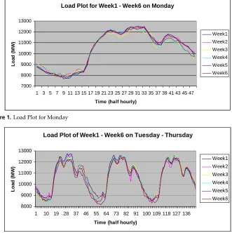
Before proceeding the forecasting process, load data need to be analyzed. Table 1 shows the average maximum and minimum demand, average energy and peak hour per day within a week. From the analysis, it can be concluded that the load characteristic among the days in a week is different. The average energy for Monday is slightly lower compared to Tuesday, Wednesday and Thursday. On the other hand, the average energy for those three days is fairly around 255MWh so that they can be clustered in a category. The average energy for Friday shows the lowest value within weekdays while the energy used for weekend is much lower than the consumption on weekdays. Comparing energy consumed on weekend, there is more consumption on Saturday rather than Sunday. Hence, the forecast will be conducted based on five day types that are:

Type 1 : Monday

Type 2 : Tuesday, Wednesday, Thursday Type 3 : Friday

(3)

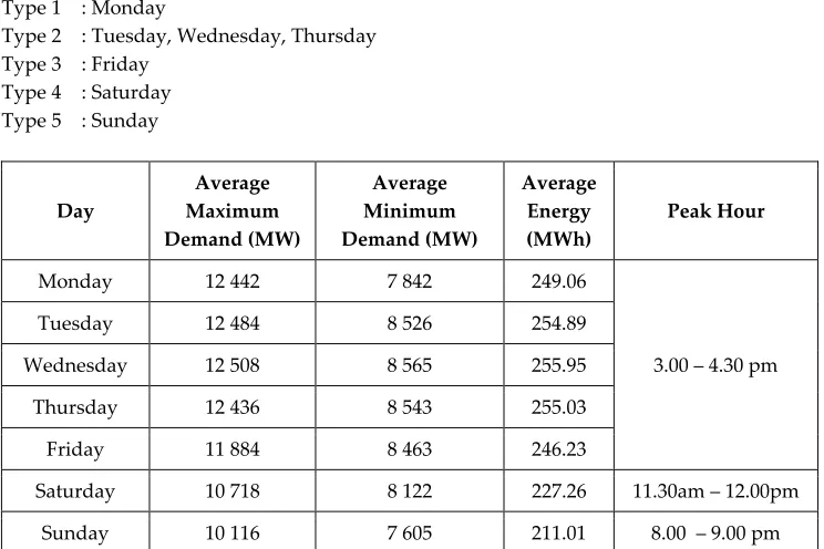
Figure 1. Load Plot for Monday

Figure 2. Load Plot for Tuesday, Wednesday and Thursday

Figure 3. Load Plot for Friday

Load Plot for Week1 - Week6 on Monday

7000

Load Plot of Week1 - Week6 on Tuesday - Thursday

8000

Load Plot of Week1 - Week6 on Friday

(4)

Figure 4. Load Plot for Saturday

Figure 5. Load Plot for Sunday

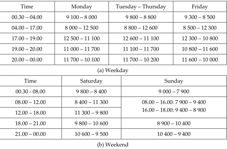
Apart from that, load plot for each day types can be observed as in Figure 1-5. Their characteristic for certain time interval can be simplified as in Table 2 (a) and (b). Referring Table 2(a) for weekday, load consumption is decreasing from time 20.00 till 00.00 and 00.30 till 04.00 where people are having some rest or sleeping at night. However, starting 04.00 till 17.00 the load consumption is increasing because people start using home appliances and go to work. The load consumption for 17.00 till 19.00 shows slight decrease as people come back to home. The next an hour show the load consumption increasing where people spend some time watching television or having a dinner. However, there are bit differences of people activities during weekend that affect load consumption.

Load Plot of Week1 - Week6 on Saturday

7000

Load Plot of Week1 - Week6 on Sunday

(5)

Time Monday Tuesday – Thursday Friday

Time Saturday Sunday

00.30 - 08.00 9 800 – 8 400 9 000 – 7 900

Table 2. Load consumption per day (MW)

Five models of SARIMA were developed in Minitab which represents the five day types. ARIMA; Autoregressive Integrated Moving Average involves the filtering steps in constructing the ARIMA model until only random noise remains. ARIMA model can be classified as seasonal or non-seasonal model. The series with seasonal repeating pattern is categorized as seasonal model or seasonal ARIMA (SARIMA) while the series with random series or no seasonal repeating trend is called as non-seasonal pattern. At least four or five seasons of the data are needed to fit the SARIMA model. Instead, ARIMA modeling identifies an acceptable model by some steps which are differencing, autocorrelation and partial autocorrelation functions. A non-seasonal ARIMA model is known as an ARIMA (p, d, q) model while a seasonal ARIMA model is named as ARIMA (P, D, Q) model where P or P is the number of autoregressive term (AR), d or D is the number of non-seasonal differences and q or Q is the number of lagged forecast errors in the prediction equation (MA). Appropriate ARIMA model is determined by identifying the p, d, q and P, D, Q parameters [10].

(6)

Value of

λ

Transformation

Table 3. Box-Cox Transformation

The last step is identifying the p, d, q and P, D, Q parameters. It started by determining the order of differencing needed to stationarize the series [10]. Normally the lowest order of differencing leads time series to fluctuates around a well-defined mean value and the spikes of ACF and PACF decays fairly rapidly to zero. After chosen appropriate order of differencing, AR and MA terms are then identified to determine whether the AR and MA terms are needed to correct any autocorrelation that remains in the differenced series.

Apart from that, the best fit of the model must meet these specifications:

a. -1.96 t-value 1.96

b. The lowest standard deviation c. Chi-Square at Lag-12 is acceptable d. -1 Parameter’s coefficient 1

Some equations related to ARIMA model are shows in (1) to (4).

The order of d can be expressed in terms of the backshift operator B as:

  d (1 B)d (1)

The seasonal backshift operator;



The seasonal difference operator;

  S (1 )

D S D

B (3)

Combining (1) and (3) yields:

 (1 ) (1d  S D)

t t

Y B B z ₍₄₎

(7)

4. SARIMA modelling

4.1. ARIMA model for monday

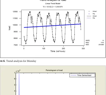
The load data on Monday for six weeks had been plotted by trend analysis. Figure 6 shows that the data is seasonal and non-stationary so the period of the data must be identified. It can be done by plotting spectral plot in MATLAB as shown in Figure 7.

Figure 6. Trend analysis for Monday

Figure 7. Spectral plot

(8)

T = 1/f (5)

Where T = period, and f = frequency

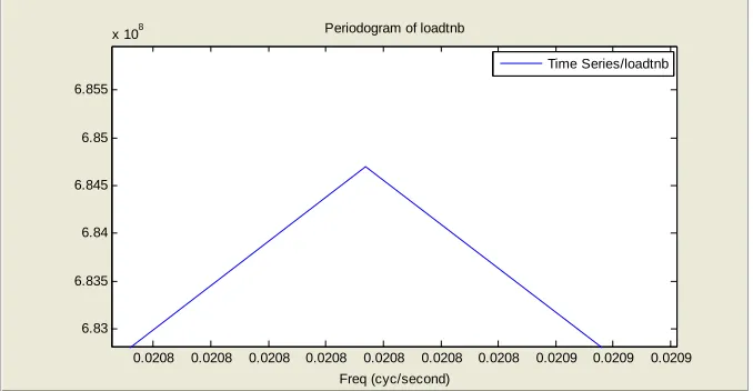
From Figure 8, the frequency was 0.0208 thus the period was approximately 48. This value was determined based on the half hourly load and is valid for all day types. Since the data was not stationary, the actual data must be transformed; depending on the value of λ.

Figure 8. Enlarged view of spectral plot

Figure 9 shows the Box-Cox Plot for Monday where the value of λ = 0.562 so the rounded value is 0.5. Hence the actual data was transformed to √Xt.

Figure 9. Box-Cox plot for Monday

0.0208 0.0208 0.0208 0.0208 0.0208 0.0208 0.0208 0.0209 0.0209 0.0209 6.83

6.835 6.84 6.845 6.85 6.855

x 108 Periodogram of loadtnb

Freq (cyc/second)

(9)

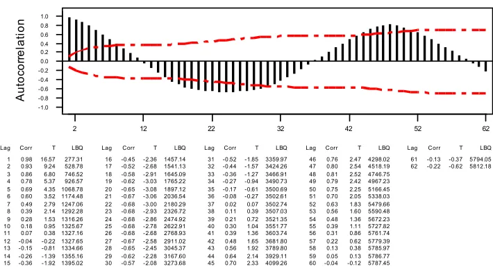
Figure 10 show bad ACF (sine-cosines' phenomenon) and PACF when all parameters are zero. It is important to ensure that all the spikes are within the boundary to be a stationary model. Then the ARIMA parameters were identified and the selected model was ARIMA (2,1,1)(0,1,1)48.

(10)

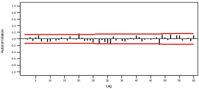
Figure 11-12 shows good ACF and PACF where the spikes decay fairly rapidly to zero. There was strong autocorrelation at lag-48 that shows the period of the data. All these steps were repeated for other day types.

5 10 15 20 25 30 35 40 45 50 55 60

ACF of Residuals for d0 D0

(with 95% confidence limits for the autocorrelations)

Figure 11. ACF Plot for ARIMA (2,1,1)(0,1,1)48 on Monday

5 10 15 20 25 30 35 40 45 50 55 60

PACF of Residuals for d0 D0

(with 95% confidence limits for the partial autocorrelations)

Figure 12. PACF Plot for ARIMA (2,1,1)(0,1,1)48 on Monday

4.2. ARIMA model for Tuesday, Wednesday and Thursday

(11)

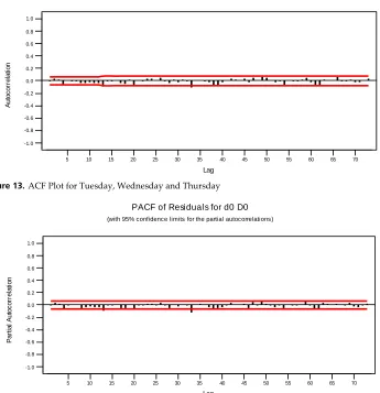
Figure 13 and 14 show good ACF and PACF for selected ARIMA model where less spikes were found outside the boundary.

70

Figure 13. ACF Plot for Tuesday, Wednesday and Thursday

5 10 15 20 25 30 35 40 45 50 55 60 65 70

Figure 14. PACF Plot for Tuesday, Wednesday and Thursday

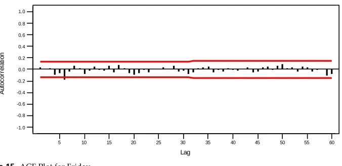
4.3. ARIMA model for Friday

(12)

Figure 15 and 16 show good ACF and PACF for Friday model with no spikes outside the

Figure 15. ACF Plot for Friday

5 10 15 20 25 30 35 40 45 50 55 60

Figure 16. PACF Plot for Friday

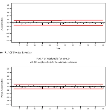
4.4. ARIMA model for Saturday

(13)

After the actual data had been transformed to ln Xt, the selected model was ARIMA

(2,1,1)(0,1,1)48.

Figure 17-18 show good ACF and PACF for Saturday with ARIMA model selected.

5 10 15 20 25 30 35 40 45 50 55 60

Figure 17. ACF Plot for Saturday

5 10 15 20 25 30 35 40 45 50 55 60

Figure 18. PACF Plot for Saturday

4.5. ARIMA model for Sunday

(14)

transformed. Box-Cox plot showed that the value of λ is 0.225 and the rounded value is 0. After the actual data had been transformed to ln Xt, the selected model was ARIMA

(0,1,1)(0,1,1)48.

Figure 19-20 show good ACF and PACF for the fitted model. The plots show less spikes outside the boundary after a differencing and good selection of p, P, q and Q.

5 10 15 20 25 30 35 40 45 50 55 60

Figure 19. ACF Plot for Sunday

5 10 15 20 25 30 35 40 45 50 55 60

(15)

5. Result and analysis

The forecasting was held for 48 points that represent a day ahead for each day types. Table 4-8 show model specifications for all day types. Referring to t-values for all models, they satisfied the condition -1.96 t-value 1.96. Besides, good standard deviations shown for all models as well as Chi-Square at Lag-12 are also acceptable. The parameters' coefficients also fulfil the condition within the range of -1 and 1.

Parameters' Coefficient t-value Standard Deviation Chi-Square at Lag-12 DF

AR 1 -0.3879

Table 4. Model Specification for Monday

AR 1 0.1962

Table 5. Model Specification for Tuesday, Wednesday and Thursday

MA 1 0.4878 SMA 48 0.6243

8.73

11.01 0.0355914 14.4 10

Table 6. Model Specification for Friday

AR 1 0.4083

Table 7. Model Specification for Saturday

MA 1 0.5746 SMA 48 0.6823

10.81

11.77 0.0596651 11.9 10

(16)

Figure 21. Actual load vs. forecasted load on Monday

Figure 22. Actual load vs. forecasted load on Tuesday, Wednesday and Thursday

Actual Load vs Forecasted Load on Monday

7000

Time (half hourly)

Loa

Actual Load vs Forecasted Load on Tuesday-Thursday

(17)

Figure 23. Actual load vs. forecasted load on Friday

Figure 24. Actual load vs. forecasted load on Saturday

Actual load vs Forecasted Load on Friday

8000

Actual Load vs Forecasted Load on Saturday

(18)

Figure 25. Actual load vs. forecasted load on Sunday

Figure 21-25 show the plots of forecasted load vs. actual load. The forecasted load plot are seems to be close as actual load plot. Mean Absolute Percentage Error (MAPE) for all day types were calculated as in (7):

 _ 

Table 9 shows the ARIMA models and their MAPEs for all day types. It can be seen that the difference order (d and D) for all models is 1which is the lowest order and the best selection. The result is considered as accurate when the MAPE is lower than 1.5% as shown for Tuesday –Thursday, Friday and Sunday models. The higher MAPE for Monday and Saturday models may caused by load or weather fluctuation.

Day ARIMA Model MAPE

Monday (2,1,1)(0,1,1)48 3.26064%

Tuesday -Thursday (1,1,1)(0,1,1)48 1.62094%

Friday (0,1,1)(0,1,1)48 1.11833 %

Saturday (2,1,1)(0,1,1)48 2.41944 %

Sunday (0,1,1)(0,1,1)48 1.07158 %

Table 9. Forecasting result for all day types

Actual Load vs Forecasted Load on Sunday

(19)

6. Conclusion

From the data analysis, load data was clustered to five day types and hence five models of SARIMA are designed. Each forecasting model is developed for each day except for Tuesday, Wednesday and Thursday which clustered as a model. Forecasting method is held by Time Series - SARIMA where it is one of data mining methods which require enough experience on determining its parameter (p,d,q,P,D,Q). Sometimes it is needs for trial and error during identifying the parameters. However, the MAPEs obtained for each day types were ranging from 1% to 3%. This new approach had improved the accuracy of forecasting compared to traditional approach of ARIMA that use only a model for all days in a week.

7. Further research

Additional input variables can be included in the forecasting process such as weather data, customers’ classes and event day; instead of only the load data. Besides, other methods may be implemented such as Neural Network, Fuzzy Logic as well as hybrid method [11].

Author details

Intan Azmira binti Wan Abdul Razak*_,

Mohd Shahrieel bin Mohd. Aras and Arfah binti Ahmad

Faculty of Electrical Engineering, UTeM, Malacca, Malaysia

Shah bin Majid

Faculty of Electrical Engineering, UTM, Johor, Malaysia

Acknowledgement

I wish to express my gratitude to honorable University (Universiti Teknikal Malaysia

Melaka- UTeM) especially to Faculty of Electrical Engineering for give the financial as well

as moral support. My special thanks also fall to Mr. Fuad Jamaluddin from Utility of Malaysia for his valuable advice and help during completion of this research. Also to all my research members that give full commitments and cooperation.

8. References

[1] I. Azmira, A. Razak, S. Majid, and H.A. Rahman, “Short Term Load Forecasting Using Data Mining Technique,” Energy Conversion and Management, 2008, pp. 139-142.

[2] “Application of Pattern Recognition and Artificial Neural Network to Load Forecasting in Electric Power System,” Pattern Recognition, 2007.

[3] P. Qingle and Z. Min, “Very Short-Term Load Forecasting Based on Neural Network and Rough Set,” Network, 2010, pp. 1132-1135.

(20)

[4] J.C. Hwang and C.S. Chen, “Customer Short Term Load Forecasting by Using Arima Transfer Function Model,” Electrical Engineering, pp. 317-322.

[5] B. Ye, N.N. Yan, C.X. Guo, and Y.J. Cao, “Identification of Fuzzy Model for Short-Term,” Evolution, 2006, pp. 1-8.

[6] S. Fan, Y.-kang Wu, W.-jen Lee, and C.-yin Lee, “Different Geographical Distributed Loads,” Systems Research, 2011, pp. 1-8.

[7] Y.H. Kareem and A.R. Majeed, “Sulaimany Governorate Using SARIMA .,” Building, 2006, pp. 1-5.

[8] “Robust Estimation of Sarima Models : Application to Short-Term Load Forecasting Yacine Chakhchoukh , Patrick Panciatici Versailles , France,” Signal Processing, 2009, pp. 77-80.

[9] J.K. Basu, D. Bhattacharyya, and T.-hoon Kim, “Use of Artificial Neural Network in Pattern Recognition,” Engineering, vol. 4, 2010, pp. 23-34.

[10]H.L. Willis, Power Distribution Planning Reference Book, North Carolina,USA: Marcel Dekker, Inc., 2004.