Journal of the Franklin Institute 350 (2013) 318–330
Robust
H
N
static output feedback controller design
for parameter dependent polynomial systems:
An iterative sums of squares approach
Matthias Krug, Shakir Saat, Sing Kiong Nguang
nDepartment of Electrical and Computer Engineering, The University of Auckland, 92019 Auckland, New Zealand
Received 22 January 2012; received in revised form 30 August 2012; accepted 10 November 2012 Available online 7 December 2012
Abstract
This paper considers the problem of designing a robust H1 static output feedback controller for polynomial systems with parametric uncertainties. Sufficient conditions for the existence of a nonlinear H1static output feedback controller are given in terms of solvability conditions of polynomial matrix inequalities. An iterative sum of squares decomposition is proposed to solve these polynomial matrix inequalities. The proposed controller guarantees that the closed-loop system is stable and theL2-gain of
the mapping from exogenous input noise to the controlled output is less than or equal to a prescribed value. Numerical examples are provided to demonstrate the validity of applied methods.
&2012 The Franklin Institute. Published by Elsevier Ltd. All rights reserved.
1. Introduction
The problem of designing a nonlinearH1controller has attracted considerable attention for
more than three decades; see for instance[1–4]. Generally speaking, the aim of anH1control
problem is to design a controller such that the resulting closed-loop control system is stable and a prescribed level of attenuation from the exogenous disturbance input to the controlled
output inL2=l2-norm is fulfilled. There are two common approaches available to address
nonlinearH1 control problems: One is based on the theory of dissipative energy [5] and
theory of differential games[1], and the other is based on the nonlinear version of the bounded
real lemma as developed in[6,7]. The underlying idea behind both approaches is the
conver-sion of the nonlinearH1 control problem into the solvability form of the Hamilton–Jacobi
equation (HJE). Unfortunately, this representation is NP-hard and it is generally very difficult to find a global solution.
www.elsevier.com/locate/jfranklin
n
Corresponding author.
The problem of static output feedback is stated as follows: given a dynamic system, find a static output feedback controller such that the closed loop system is stable. The formulation to obtain a static output controller can be used to design a full order dynamic
controller, but the converse is not true [8]. An iterative linear matrix inequality (ILMI)
procedure to compute the static output feedback gain for linear systems can be found in
[9]. The result has been extended to nonlinear systems using Takagi–Sugeno (TS) fuzzy
model to approximate the system’s nonlinearities in[10]. In there, the ILMI methodology
has been used to solve bilinear matrix inequalities. Further, in [11]the ILMI method is
used to obtain a nonlinearH1static output controller for TS fuzzy models. The authors
assume that the premises variables are bounded, thus implying that the state variables are also bounded. Additionally, the algorithm requires that the Lyapunov function to be of a quadratic form.
Using the so-called sum of squares (SOS) decompositions of polynomial terms, a computational relaxation of the solvability conditions of the HJE has been presented in
[12]. In detail, the SOS decomposition uses Gram Matrix methods to efficiently transform
the HJE, into LMIs[13]. These can in turn be solved in polynomial time with semidefinite
programming (SDP) [14,15]. There exist several freely available toolboxes to formulate
these problems in Matlab, for example SOSTOOLS [16], YALMIP [17], CVX[18], and
GloptiPoly [19]. Whereas SOSTOOLS is specifically designed to address polynomial
non-negativity problems, the latter toolboxes have more functionalities, such as modules to solve the dual of the SOS problem and the moment problem.
In recent years, several approaches utilizing SOS decompositions to achieve nonlinearH1
control have been presented, e.g. [20–25]. The systems discussed are represented in a state
dependent linear-like form and the authors assumed that the control input matrix has some zero rows. Further, it was assumed that the state dynamics are not directly affected by the control input, that is the Lyapunov function can only depend on states whose corresponding rows in control matrix are zero. These assumptions, however, lead to conservatism in the controller design.
To the best of authors’ knowledge, there is no general result forH1static output feedback
controller design for polynomial systems. Even though[24]addressed this problem, it uses the
same assumption as[23], i.e. the corresponding rows of the control matrix has some zeros rows
and Lyapunov function only depends on states whose corresponding rows in control matrix are zero. By making this assumption, one can avoid non-convex expressions in the static output feedback design, but introduces conservatism in the design. The main contributions of this paper can be summarized as follows:
The proposed controller design avoids rational static output feedback controllersresulting from the inversion of the Lyapunov function.
The Lyapunov function does not require to be a function of states whose correspondingrows in control matrix are zeroes.
The rest of this paper is organized as follows: Section 2 provides the preliminaries and
notations used throughout the rest of the paper. The main results are highlighted inSection 3.
Then, the validity of the presented algorithm is illustrated with examples in Section 4.
2. Preliminaries and notations
In this section, we introduce the notation that will be used in the rest of the paper. Further-more, we provide a brief review on SOS decomposition. For a more elaborate description of the SOS decompositions and their applications in control, see for example[12,26].
2.1. Notations
Let Rbe the set of real numbers andRn be the n-dimensional real space. Furthermore,
letInrepresent the identity matrix of sizenn. For a square matrixQ,Qg0ðQk0Þis used to express its positive (semi)definiteness.
When talking about partial derivatives of a Lyapunov function V(x) innvariables, we
denote@VðxÞ=@xas a row vector, i.e.@VðxÞ=@x¼ ½@VðxÞ=@x1,@VðxÞ=@x2,. . .,@VðxÞ=@xn. ‘‘n’’ is used to represent transposed symmetric matrix entries. InSection 3.2, we use½i
t
as an index for the current iterationtof the sub-matrix i.
2.2. SOS decomposition
Definition 2.1. A multivariate polynomialf(x), x2Rn, is a sum of squares if there exist polynomialsfiðxÞ,i¼1,. . .,msuch that
fðxÞ ¼ X m
i¼1
fi2ðxÞ: ð1Þ
FromDefinition 2.1, it is clear that the set of SOS polynomials innvariables is a convex
cone, and it is also true (but not obvious) that this convex cone is proper [27]. If a
decomposition off(x) in the above form can be obtained, it is clear thatfðxÞZ0,8x2Rn. The converse, however, is generally not true.
The problem of finding the right hand side of Eq.(1)can be formulated in terms of the
existence of a positive semidefinite matrixQsuch that the following proposition holds:
Proposition 2.1 (Parrilo[12]). Let f(x)be a polynomial in x2Rnof degree2d.Let Z(x)be a column vector whose entries are all monomials in x with degreerd.Then,f(x)is said to be SOS if and only if there exists a positive semidefinite matrix Q such that
fðxÞ ¼ZðxÞTQZðxÞ: ð2Þ
In general, determining the non-negativity off(x) fordegðfÞZ4 is a NP-hard problem[28,29].
Proposition 2.1 provides a relaxation to formulate non-negativity conditions on polynomials that is computational tractable. A more general formulation of this transformation for sym-metric polynomial matrices is given in the following proposition:
Proposition 2.2 (Prajna et al.[20]). Let F(x) be an NN symmetric polynomial matrix of degree2d in x2Rn.Furthermore,let Z(x)be a column vector whose entries are all monomials in x with a degree no greater than d,and consider the following conditions:
(1) FðxÞk0 for all x2Rn;
(3) there exists a positive semidefinite matrix Q such that vTFðxÞv¼ ðvZðxÞÞTQ
ðvZðxÞÞ, withdenoting the Kronecker product.
F(x)being a SOS implies FðxÞk0.The converse,however,is generally not true. Furthermore, Statements(2)and(3)are equivalent.
3. Main results
In this section, we start with the derivation of aH1controller for polynomial systems without parametric uncertainties. The results are subsequently extended to the robust control synthesis.
3.1. H1control of polynomial systems without parametric uncertainties
Consider the following dynamic model of a polynomial system:
_
x¼AðxÞ þBuðxÞuþBoðxÞo, y¼CyðxÞ,
z¼CzðxÞ þDzðxÞu, ð3Þ
where o2Rp is the disturbance input and z is the output to be regulated.AðxÞ, CyðxÞ,
CzðxÞ are polynomial vectors and BuðxÞ, BoðxÞ, DzðxÞ are polynomial matrices of
appropriate dimensions. The objective of static output feedbackH1 control is to find a
controller K(y) such that the system(3)with
u¼KðyÞ ð4Þ
is asymptotically stable and the L2 gain from the disturbance input to the controlled
output is less than a prescribed valueg40, that is,
Z 1
0
zTz dtrg2
Z 1
0
oTodt: ð5Þ
Theorem 3.1. The polynomial system (3) is stabilizable with a prescribed H1performance g40via a static output feedback controller(4)if there exist a polynomial function V(x)and a
polynomial matrix K(y)such that8xa0
VðxÞ40 ð6Þ
and
@VðxÞ @x AðxÞ
1 4
@VðxÞ @x BuðxÞB
T uðxÞ
@VTðxÞ
@x þ
1 2
@VðxÞ @x BoðxÞ
1
g2 1 2
@VðxÞ @x BoðxÞ
T
þ 12@V@xðxÞBuðxÞ þKTðyÞ
1
2
@VðxÞ
@x BuðxÞ þK T
ðyÞ
T
þ ðCzðxÞ þDzðxÞKðyÞÞTðCzðxÞ þDzðxÞKðyÞÞo0: ð7Þ
Proof. Note that for8xa0
_
VðxÞ ¼@VðxÞ
r@VðxÞ
Integrating both sides of the inequality yields
Z 1
Hence Eq.(5)holds and the H1 performance is fulfilled.
To prove that the closed-loop system(3)with Eq.(4)is asymptotically stable, we set the
disturbance oðtÞ ¼0. From Eq. (9), we learn that V_ðxðtÞÞo0, hence, by the Lyapunov
stability theorem the closed-loop system(3) with Eq.(4) is asymptotically stable. &
The separation of the Lyapunov function and the controller of the H1 static output
feedback problem in Eq.(7)is the first step in bringing the problem in a more suitable form
for numerical methods. However, it cannot be expressed as a state-dependent LMI, due to
the negative term 1
4ð@VðxÞ=@xÞBuðxÞB T
uðxÞ@VTðxÞ=@x. To accommodate this negative
term, an additional design polynomial vectorEðxÞof appropriate dimension is introduced.
for anyEðxÞand@VðxÞ=@xof the same dimension, we obtain
Theorem 3.2. The polynomial system (3) is stabilizable with a prescribed H1performance g40via a static output feedback controller(4),if there exist a polynomial function V(x),a
polynomial vector EðxÞof appropriate dimensions, and a polynomial matrix K(y)satisfying the following condition for8xa0
VðxÞ40, ð11Þ
Proof. It is obvious that using Eq.(10)in Eq.(7)yields
@VðxÞ
thus representing a sufficient condition forH1stability. Applying Schur Complement, one
can verify Eq.(12). &
The term1
2EðxÞBuðxÞBTuðxÞ@VTðxÞ=@xmakes Eq.(12)non-convex, hence the inequality cannot be solved directly by SOS decomposition. Hence, we propose the following iterative
ISOS algorithm forH1static output feedback control of polynomial systems.
Step1: Linearize system (3) and set o¼0. Use the static output feedback approach
described in[9]to find a solution to the linearized problem without disturbance. Set
t¼1,E1ðxÞ ¼xTP,V0¼xTPx.
Step2: Solve the following SOS optimization problem in Vt(x) and Kt(y) with fixed
auxiliary polynomial vectorEtðxÞand some positive polynomialsl1ðxÞandl2ðxÞ:
feedback control problem of polynomial systems. Terminate the algorithm.
Step3: Set t¼tþ1 and solve the following SOS optimization problem in Vt(x), Kt(y),
with Z(x) as in Proposition 2.2 and the SOS decomposition of the Lyapunov
functionVtðxÞ ¼ZðxÞTQtZðxÞ,EtðxÞ ¼Et1ðxÞas well as some positive polynomials
Step4: Solve the following feasibility problem withv2 2Rnþ1 and some positive tolerance
Step5: The system (3) may not be stabilizable with H1 performance gby static output
feedback(4). Terminate the algorithm. &
Remark 3.1. The term1
2EðxÞBuðxÞBTuðxÞ@VTðxÞ=@xmakes Eq.(12)non-convex, hence the inequality cannot be solved directly by SOS decomposition. If, however, the auxiliary
polynomial vector EðxÞ is fixed, Eq. (12) becomes convex and can be solved efficiently.
Unfortunately, fixing EðxÞ generally does not yield a feasible solution. Therefore, we
introduceatVt1ðxÞin Eq.(15)to relax the SOS decomposition in Eq.(12)and makes it
feasible. This corresponds to the following Lyapunov inequalities:
VtðxÞ40,
_
VtðxÞratVt1ðxÞ:
Similar Lyapunov inequalities can be obtained for Eq. (16). If a in Eq. (15) or (16) is
negative, then we conclude the system(3)with Eq.(4) is stable.
Step 1 is the initialization of the iterative algorithm and necessary to find an initial value
of E1ðxÞ to use in the following iterations. The optimization problem in Step 2 is a
generalized eigenvalue minimization problem and guarantees the progressive reduction of
at. Meanwhile, Step 3 ensures convergence of the algorithm. Step 4 updatesEðxÞand checks whether the iterative algorithm stalls, i.e. the gap between EðxÞ and @VðxÞ=@x is smaller than some positive tolerance functiondðxÞ.
Note that the iterative algorithm increases the iteration variable t twice per cycle (in
Steps 3 and 4). This is done to avoid confusion with the indexes.
3.2. Robust stability synthesis
The results presented in the previous section assume that all system parameters are known exactly. In this section, we extend the results to polynomial systems with parametric uncertainties.
Consider the following system:
_
x¼Aðx,yÞ þBuðx,yÞuþBoðx,yÞw,
y¼Cyðx,yÞ,
z¼Dzðx,yÞ þDzðx,yÞu, ð17Þ
where the matricesðx,yÞare defined as follows:
Aðx,yÞ ¼ X
q
i¼1
AiðxÞyi, Buðx,yÞ ¼
X
q
i¼1
BuiðxÞy, Boðx,yÞ ¼ X
q
i¼1
BoiðxÞy,
Cyðx,yÞ ¼
X
q
i¼1
CyiðxÞy, Czðx,yÞ ¼ X
q
i¼1
CziðxÞy, Dzðx,yÞ ¼ X
q
i¼1
DziðxÞy: ð18Þ
y¼ fy1,. . .,yqgT 2Rq is the vector of constant uncertainty and satisfies
y2Y9 y2Rq:yiZ0,i¼1,. . .,q,X
q
i¼1
yi¼1
( )
We further define the following parameter dependent Lyapunov function:
VðxÞ ¼ X q
i¼1
ViðxÞyi: ð20Þ
With the results from the previous section, we have the main result for the robust H1
static feedback controller design for polynomial systems with parametric uncertainties.
Theorem 3.3. The polynomial system with parametric uncertainties(17)is stabilizable with a prescribed H1performanceg40via a static output feedback(4)if there exist a polynomial
function V(x) as in Eq. (20), a polynomial vector EðxÞ ¼Pq
Proof. This theorem follows directly from Theorem 3.2. &
The same ISOS algorithm given inSection 3.1can be employed to solve Eq.(23):
4. Numerical example
In this section, we will provide two design examples to demonstrate the validity of
the proposed H1 static output feedback controller design for polynomial systems with
parametric uncertainties.
4.1. Lorenz Chaotic System
The dynamics of the Lorenz Chaotic System can be described as follows:
_
a parametric uncertainty withb2 ½0:1,0:1:
1þx22þx23Þ. We initially choose quadratic Lyapunov function candidates and set the polynomial static output feedback controller to be of the formKðyÞ ¼m1yþm2y2. The ISOS algorithm terminates without obtaining a feasible solution, thus we increase the degree
of the Lyapunov function candidates to 4. This yields a feasible solution withm20, therefore
indicating thatm2¼0 may also be a feasible solution. After four iterations, the following static output feedback controller withg¼1:567 is obtained:
KðyÞ ¼ 20:353y: ð26Þ
The corresponding Lyapunov functions are
VðxÞ ¼1:8378x41þ0:2204x31x2þ2:3156x21x22þ0:7371x21x232:0176x21x3þ59:7839x21
Fig. 1 shows the closed-loop responses of the Lorenz Chaotic System with initial conditions
x0¼ ½20,10,20Tand a random white noise disturbanceowith power spectrum density of 1
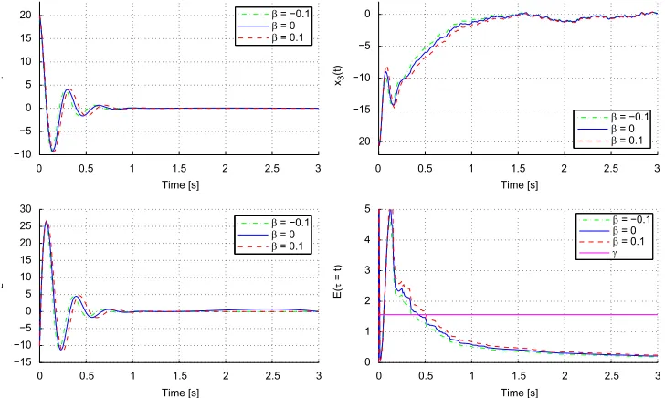
Consider the polynomial system from[24], whereb2 ½1,1:
_
3y3 and initially look for Lyapunov function candidates of degree 4. The ISOS
withH1 performanceg¼1:514 is obtained:
KðyÞ ¼0:380y: ð29Þ
The corresponding with Lyapunov functions are
V¼0:09585x41þ0:0476x13x2þ0:0455x31þ0:0340x 2 1x
2
2þ0:0718x
2
1x2þ0:2812x21 þ0:0934x1x320:0362x1x220:1322x1x2þ0:08515x420:0558x32þ0:5756x22 þbð0:0125x41þ0:0388x31x20:0109x310:0146x21x220:0134x21x20:0005x21 0:0862x1x32þ0:024x1x220:0238x1x20:03675x420:0132x
3
20:0454x 2
2Þ: ð30Þ
The smallestgobtained in this paper is 1.514, which is smaller than 1.8071 obtained in[24]. It is noteworthy that thisgis achieved with alinearcontroller compared to thepolynomialcontroller obtained in[24].Fig. 2shows that the closed-loop system responses with the initial conditions
arex0¼ ½10,10T and the disturbance is modeled by Gaussian white noise with power density
spectrum of 0.01. After 20 s,EðtÞtends to a value which is less thanð1:514Þ2.
5. Conclusion
A novel approach for designing a nonlinear H1 static output feedback controller for
polynomial systems with parametric uncertainties has been proposed. Sufficient conditions
for the existence of a nonlinear H1 static output feedback controller are derived and
expressed in terms of polynomial matrix inequalities. In order to solve these polynomial matrix inequalities, an iterative sum of squares decomposition has been proposed. The novelties of our approach are (1) the proposed controller design avoids rational static output feedback controllers resulting from the inversion of the Lyapunov function and (2)
the Lyapunov function does not require to be a function of states whose corresponding rows in control matrix are zeroes. Through simulation examples, we have shown that our results are less conservative than the results given in[24].
Acknowledgments
The authors gratefully acknowledge the support in part by The University of Auckland, Technical University of Malaysia Malacca (UTeM), and Government of Malaysia Scholarship.
References
[1] J. Ball, J. Helton,H1control for nonlinear plants: connections with differential games, in: Conference on Decision and Control, 1989, pp. 956–962.
[2] T. Bas-ar, G.J. Olsder, Dynamic Noncooperative Game Theory, Academic Press, London, New York, 1995. [3] A. van der Schaft, L2-gain analysis of nonlinear systems and nonlinear state-feedbackH1control, IEEE
Transactions on Automatic Control 37 (6) (1992) 770–784.
[4] A. Isidori, A. Astolfi, Disturbance attenuation andH1-control via measurement feedback in nonlinear systems, IEEE Transactions on Automatic Control 37 (9) (1992) 1283–1293.
[5] T. Bas-ar, Optimum performance levels for minimax filters, predictors and smoothers, Systems & Control Letters 16 (5) (1991) 309–317.
[6] D.J. Hill, P.J. Moylan, Dissipative dynamical systems: basic input–output and state properties, Journal of the Franklin Institute 309 (5) (1980) 327–357.
[7] J.C. Willems, Dissipative dynamical systems. Part i: general theory, Archive for Rational Mechanics and Analysis 45 (1972) 321–351.
[8] V. Syrmos, C. Abdallah, P. Dorato, K. Grigoriadis, Static output feedback—a survey, Automatica 33 (2)
(1997) 125–137.
[9] Y.-Y. Cao, J. Lam, Y.-X. Sun, Static output feedback stabilization: an ILMI approach, Automatica 34 (12) (1998) 1641–1645.
[10] D. Huang, S.K. Nguang, Static output feedback controller design for fuzzy systems: an ILMI approach, Journal of Information Sciences 177 (14) (2007) 3005–3015.
[11] D. Huang, S.K. Nguang, RobustH1static output feedback control of fuzzy systems: an ILMI approach, IEEE Transactions on Systems, Man, and Cybernetics, Part B: Cybernetics 36 (1) (2006) 216–222. [12] P.A. Parrilo, Structured Semidefinite Programs and Semialgebraic Geometry Methods in Robustness and
Optimization, Ph.D. Thesis, California Institute of Technology, May 2000.
[13] V. Powers, T. W ¨ormann, An algorithm for sums of squares of real polynomials, Journal of Pure and Applied Algebra 127 (1) (1998) 99–104.
[14] L. Vandenberghe, S.P. Boyd, Semidefinite programming, SIAM Review 38 (1) (1996) 49–95.
[15] S.P. Boyd, L.E. Ghaoui, E. Feron, V. Balakrishnan, Linear matrix inequalities in system and control theory, SIAM, Philadelphia, 1994.
[16] S. Prajna, A. Papachristodoulou, P.A. Parrilo, Introducing SOSTOOLS: a general purpose sum of squares programming solver, in: Conference on Decision and Control, vol. 1, 2002, pp. 741–746.
[17] J. Lofberg, YALMIP: a toolbox for modeling and optimization in Matlab, in: IEEE International Symposium on Computer Aided Control Systems Design, 2004, pp. 284–289.
[18] M. Grant, S. Boyd, Graph implementations for nonsmooth convex programs, in: V. Blondel, S. Boyd, H. Kimura (Eds.), Recent Advances in Learning and Control, Lecture Notes in Control and Information Sciences, Springer Verlag, 2008, pp. 95–110.
[19] D. Henrion, J.-B. Lasserre, J. L ¨ofberg, GloptiPoly 3: moments, optimization and semidefinite programming, Optimization Methods and Software 24 (4) (2009) 761–779.
[20] S. Prajna, A. Papachristodoulou, F. Wu, Nonlinear control synthesis by sum of squares optimization: a Lyapunov-based approach, in: Asian Control Conference, vol. 1, 2004, pp. 157–165.
[21] A. Papachristodoulou, S. Prajna, On the construction of Lyapunov functions using the sum of squares decomposition, in: Conference on Decision and Control, vol. 3, 2002, pp. 3482–3487.
[22] H.-J. Ma, G.-H. Yang, Fault-tolerant control synthesis for a class of nonlinear systems: sum of squares optimization approach, International Journal of Robust and Nonlinear Control 19 (5) (2009) 591–610. [23] D. Zhao, J. Wang, An improvedH1synthesis for parameter-dependent polynomial nonlinear systems using
SOS programming, in: American Control Conference, 2009, pp. 796–801.
[24] D. Zhao, J.-L. Wang, Robust static output feedback design for polynomial nonlinear systems, International Journal of Robust and Nonlinear Control 20 (14) (2010) 1637–1654.
[25] P. Li, J. Lam, G. Chesi, On the synthesis of linearH1filters for polynomial systems, Systems & Control Letters 61 (1) (2012) 31–36.
[26] G. Chesi, A. Garulli, A. Tesi, A. Vicino, Homogeneous Polynomial Forms for Robustness Analysis of Uncertain Systems, Springer, Berlin, 2009.
[27] H. Hindi, A tutorial on convex optimization, in: American Control Conference, vol. 4, 2004, pp. 3252–3265. [28] A. Papachristodoulou, S. Prajna, A tutorial on sum of squares techniques for systems analysis, in: American
Control Conference, vol. 4, 2005, pp. 2686–2700.