MLA makes no representation as to the accuracy of any information or advice contained in this document and excludes all liability, whether in contract, tort (including negligence or breach of statutory duty) or otherwise as a result of reliance by any person on such information or advice. © Meat and Livestock Australia (2003)
Project LIVE.116
Final Report prepared for MLA and Livecorp
by:
Maunsell Australia Pty Ltd
12 Cribb Street, Milton QLD 4064
Published by Meat & Livestock Australia Ltd
ABN 39 081 678 364
ISBN 1 74036 443 0
December 2003
LIVE.116
Development of a Heat Stress Risk
Management Model
Final Report
Authorised
Revision Revision Date Details
Name/Position Signature
A 04/03/03 Unchecked Milestone 2 Draft for Review and Comments
Dr Conrad Stacey Technical Director
CHBS
B 06/03/03 Issued for Milestone 2 Review at Industry Consultative Committee Meetings
Dr Conrad Stacey Technical Director
CHBS
C 17/4/03 Re-write to Milestone 4 status in draft form
Dr Conrad Stacey Technical Director
CHBS
D 14/05/03 Release for Use by Industry Dr Conrad Stacey
Technical Director
CHBS
E 21/10/03 Final Version Dr Conrad Stacey
Technical Director
CHBS
F 03/12/03 Revised Final Version Dr Conrad Stacey
Table of Contents
Executive Summary 8
1 Introduction 9
1.1 Background 9
1.2 Scope and Objectives 9
1.3 Project Progress 10
1.4 A Quick Look at Outcomes 10
1.5 Recommendations for Further Work 12
1.5.1 Weather 12
1.5.2 Animal Parameters 12
1.5.3 Vessel Ventilation 13
2 Weather 13
2.1 Middle East Weather 13
2.1.1 Data Sources and Quality 13
2.1.2 General Temperature Observations 14
2.2 Voyage Weather 14
2.2.1 Data Source and Quality 16
2.3 Use of Voyage and Destination Weather 17
2.4 Departure Ports 19
3 Animal Parameters 23
3.1 Appropriate Terminology and Definitions 23 3.2 Evaluating the Heat Stress Threshold and Mortality Limit 24
3.3 Scaling HST and ML 34
3.3.1 Weight Scaling 35
3.3.2 Acclimatisation 35
3.3.3 Coat 36
3.3.4 Condition 36
3.4 Thermal Modelling 37
3.4.1 Overview 37
3.4.2 Details 37
3.5 Validation from a Voyage 38
3.5.1 Comparison of Actual and ‘Predicted’ Mortality 38
3.5.2 Relative Mortality 38
4 Ship Parameters 39
5 Open Deck Conditions 39
5.1 Animal Representation 40
5.2 Deck Representation 40
5.3 Summary of CFD Results 40
5.4 Deck and Crosswind Scaling 43
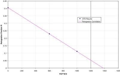
5.4.1 A Model of Reingestion 43
5.4.2 Natural Convection 44
5.4.3 Crosswind Scaling 47
5.4.4 Minimum Required Crosswind 47
6 Closed Deck Risk Estimate Calculation 48
6.1 Deck Wet Bulb Temperature Rise 48
6.2 Statistical Combination of Weather and Animal Parameters 49
6.2.1 Expected Mortality Rate 49
6.2.2 Probability of 5% Mortality 49
6.2.3 Duration of Exposure 50
7 Open Deck Risk Management 51
7.1 Overall Approach 51
7.2.1 General comments 52
7.2.2 Red Sea Ports 53
7.2.3 Gulf Ports 53
7.3 Open Deck Operation Guidelines 54
7.3.1 Effective Crosswind 54
7.3.2 Effective PAT in Still Air 55
7.3.3 Effective PAT in Light Crosswinds 55
7.3.4 PAT with Strong Crosswinds 56
7.3.5 Operating Guidelines 56
8 Software 57
8.1 Function 57
8.2 Platform 57
References 58
Appendix A Weather Details 59
A.1 Discharge Port Climatology 59
A.2 Departure Port Wet Bulb Climatology 62
Appendix B Animal Details 74
B.1 Key Terminology: A Brief Overview 74 B.2 Heat tolerance in relevant species 76
B.2.1 Published Information 76
B.2.2 Experimental Information 76
B.2.3 Voyage Investigations 84
B.3 Additional Questions Relevant to the Risk Management Model 87 B.3.1 Aspects of the Physiology of Sweating 87 B.3.2 Aspects of the Physiology of Respiratory Evaporation 87
Appendix C Computational Fluid Dynamics (CFD) 88
C.1 Cattle Parameters 88
C.2 Sheep Parameters 89
C.3 Deck Parameters 90
C.4 Domain Parameters 90
C.5 CFD Parameters 91
C.6 Analysis and Data Manipulation 91
C.7 Accuracy 92
C.8 Model Summary 92
Appendix D Scaling Open Deck Results 124
D.1 Reingestion 124
D.2 Natural Convection 126
List of Figures
Figure 1.1 Allowable Stocking Fraction for 300kg Bos indicus, fat score 3, acclimatised to 15oC wet
bulb... 11
Figure 1.2 Allowable Stocking Fraction for 300kg Bos taurus, fat score 3, acclimatised to 15oC wet bulb, mid season coat ... 11
Figure 1.3 Allowable Stocking Fraction for 40kg Adult Merinos, fat score 3, acclimatised to 15oC wet bulb, shorn... 12
Figure 2.1 Indian Ocean Weather Zones Map ... 18
Figure 2.2 Australian Acclimatisation Zone Map with Average January (top number) and July (bottom number) Wet Bulb Temperatures at Various Sites ... 20
Figure 2.3 Australian Weather Zones Map ... 21
Figure 2.4 Acclimatisation Wet Bulb Temperatures by Zone and Month... 23
Figure 3.1 Beta Function Probability Distribution – Bos taurus - beef ... 30
Figure 3.2 Beta Function Probability Distribution – Bos taurus - dairy... 31
Figure 3.3 Beta Function Probability Distribution – Bos indicus... 31
Figure 3.4 Beta Function Probability Distribution – 25% Bos indicus... 32
Figure 3.5 Beta Function Probability Distribution – 50% Bos indicus... 32
Figure 3.6 Beta Function Probability Distribution – Merino - Adult ... 33
Figure 3.7 Beta Function Probability Distribution – Merino - Lamb... 33
Figure 3.8 Beta Function Probability Distribution – Awassi - Adult ... 34
Figure 3.9 Beta Function Probability Distribution – Awassi - Lamb ... 34
Figure 3.10 Variation of Acclimatisation Factor with Acclimatising Wet Bulb Temperature... 36
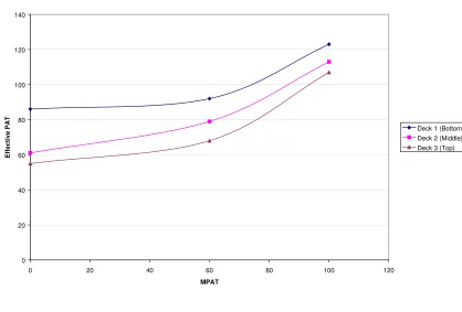
Figure 5.1 Summary of CFD Data for Cattle Decks. Variation of Effective PAT with Mechanical PAT ... 41
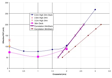
Figure 5.2 Variation of Effective PAT with Crosswind for Cattle Decks ... 41
Figure 5.3 Summary of CFD Data for Sheep Decks. Variation of Effective PAT with Mechanical PAT ... 42
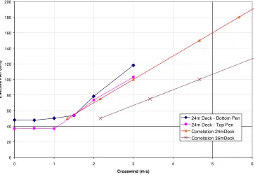
Figure 5.4 Variation of Effective PAT with Crosswind for Sheep Decks ... 42
Figure 5.5 Effective PAT Reduction by Reingestion ... 43
Figure 5.6 Reingestion Fraction Interpreted from CFD and Correlated to PAT, Deck Width and Deck Height ... 44
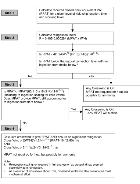
Figure 5.7 Crosswind Assessment Flowsheet for Cattle Decks ... 45
Figure 5.8 Crosswind Assessment Flowsheet for Double-tiered Sheep Decks... 46
Figure B.1 SBMR.002 - All Voyages Respiration Rate against Wet Bulb Temperature ... 78
Figure B.2 SBMR.002 - Effect of Acclimatisation on Respiration Response ... 78
Figure B.3 Respiratory Response of Sheep and Goats to Wet Bulb Temperature (from SBMR.002)79 Figure B.4 Core Temperature Response During LIVE.209 Experiments ... 79
Figure B.5 Changes in Mean Respiratory Rate (from LIVE.209)... 81
Figure B.6 Changes in Mean Core Body Temperature Changes (from LIVE.209)... 81
Figure B.7 Voyage 1 (comparing B wethers [orange symbols], Muscat wethers [blue] and Merino wether lambs [green]) ... 82
Figure B.8 Voyage 2 (a range of Merino wethers) ... 83
Figure B.9 Correlation of Body Temperature and Wet Bulb Temperature... 83
Figure B.10 Wet Bulb Temperatures and Mortality on Voyage 1 of MV Becrux... 85
Figure B.11 Wet Bulb Temperatures and Mortality Rate among Sheep on Voyage 1 of MV Becrux 86 Figure C.1 Schematic of Cattle Representation...88
Figure C.2 Schematic of Sheep Representation... 89
Figure C.3 Representative Cow Geometry used for CFD Study ... 94
Figure C.4 Representative Sheep Geometry used for CFD Study ... 95
Figure C.5 Dry Bulb Temperature Vertical Plane... 96
Figure C.6 Dry Bulb Temperature Horizontal Plane... 97
Figure C.7 Wet Bulb Temperature Vertical Plane ... 98
Figure C.8 Mass Fraction of Water Vertical Plane ... 99
Figure C.10 Dry Bulb Temperature Horizontal Plane... 101
Figure C.11 Wet Bulb Temperature Vertical Plane ... 102
Figure C.12 Wet Bulb Temperature Vertical Plane ... 103
Figure C.13 Mass Fraction of Water Vertical Plane ... 104
Figure C.14 Layout of 2 tier sheep model - 24m deck ... 105
Figure C.15 Layout of 2 tier sheep model ... 106
Figure C.16 Dry Bulb Temperature Vertical Plane... 107
Figure C.17 Dry Bulb Temperature Vertical Plane... 108
Figure C.18 Wet Bulb Temperature Vertical Plane ... 109
Figure C.19 Wet Bulb Temperature Vertical Plane ... 110
Figure C.20 Wet Bulb Temperature Horizontal Plane Through Top Tier... 111
Figure C.21 Mass Fraction of Water Vertical Plane Through Top Tier ... 112
Figure C.22 Air Velocity Vertical Plane Through Top Tier ... 113
Figure C.23 Wet Bulb Temperature Sample Point Location ... 114
Figure C.24 Contours of Wet Bulb Temperature along Pen Centreline – Forced 30 PAT, 0.0m/s Crosswind, 24m Wide Deck ...114
Figure C.25 Contours of Wet Bulb Temperature along Pen Centreline – Forced 40 PAT, 0.0m/s Crosswind, 24m Wide Deck ...115
Figure C.26 Contours of Wet Bulb Temperature along Pen Centreline – Forced 40 PAT, Closed Deck, 24m Wide Deck... 115
Figure C.27 Contours of Wet Bulb Temperature along Pen Centreline – Forced 40 PAT, 1.0m/s Crosswind, 24m Wide Deck ...116
Figure C.28 Contours of Wet Bulb Temperature along Pen Centreline – Forced 40 PAT, 1.0m/s Crosswind, 36m Wide Deck ...116
Figure C.29 Contours of Wet Bulb Temperature along Pen Centreline – Forced 60 PAT, 0.0m/s Crosswind, 24m Wide Deck ...117
Figure C.30 Contours of Wet Bulb Temperature along Pen Centreline – Forced 60 PAT, Closed Deck, 24m Wide Deck... 117
Figure C.31 Contours of Wet Bulb Temperature along Pen Centreline – Forced 60 PAT, 1.0m/s Crosswind, 24m Wide Deck ...118
Figure C.32 Contours of Wet Bulb Temperature along Pen Centreline – Forced 60 PAT, vents directed 45o downwards , 0.0m/s Crosswind, 24m Wide Deck ... 118
Figure C.33 Contours of Wet Bulb Temperature along Pen Centreline – Forced 90 PAT, 0.0m/s Crosswind, 24m Wide Deck ...119
Figure C.34 Contours of Wet Bulb Temperature along Pen Centreline – Forced 150 PAT, 0.0m/s Crosswind, 24m Wide Deck ...119
Figure C.35 Contours of Wet Bulb Temperature along Pen Centreline – 0m/s Crosswind (right to left), 24m Wide Deck... 120
Figure C.36 Contours of Wet Bulb Temperature along Pen Centreline – 0m/s Crosswind (right to left), 36m Wide Deck... 120
Figure C.37 Contours of Wet Bulb Temperature along Pen Centreline – 0.5m/s Crosswind (right to left), 24m Wide Deck... 121
Figure C.38 Contours of Wet Bulb Temperature along Pen Centreline – 1.0m/s Crosswind (right to left), 24m Wide Deck... 121
Figure C.39 Contours of Wet Bulb Temperature along Pen Centreline – 1.5m/s Crosswind (right to left), 24m Wide Deck... 122
Figure C.40 Contours of Wet Bulb Temperature along Pen Centreline – 2.0m/s Crosswind (right to left), 24m Wide Deck... 122
Figure C.41 Contours of Wet Bulb Temperature along Pen Centreline – 3.0m/s Crosswind (right to left), 24m Wide Deck... 123
List of Tables
Table 2.1 Idealized “Normal” Wet Bulb Probability Distributions (mean ± standard deviation) ... 19
Table 2.2 Acclimatisation Wet Bulb Temperatures by Zone and Month ... 22
Table 3.1 Original and Inferred Cattle Parameters ... 26
Table 3.2 Original and Inferred Sheep Parameters ... 27
Table 3.3 Scaling Factors... 28
Table 3.4 Base Heat Stress Threshold and Mortality Limit Values for the ‘Standard’ Animals ... 29
Table 7.1 Crosswind factor (sin(wind angle))... 55
Table 7.2 Minimum Crosswind for Through Ventilation ... 55
Table 7.3 Effective Natural PAT for Crosswinds Greater than in Table 7.2 (no re-ingestion from decks below) ... 56
Table 7.4 Effecting PAT (m/hr) with Crosswind ...56
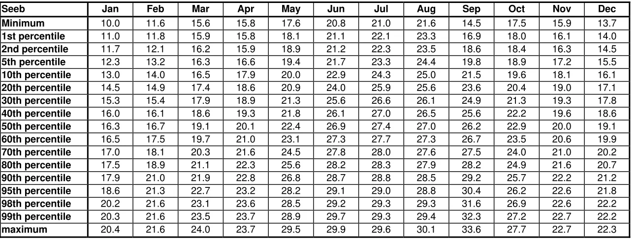
Table A.1 Wet Bulb Distribution for Seeb (Muscat) (oC) for January through December ... 64
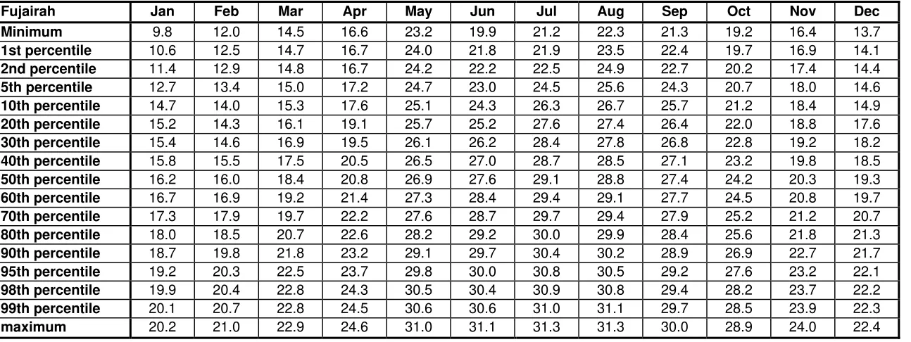
Table A.2 Wet Bulb Distribution for Fujairah (oC) for January through December... 65
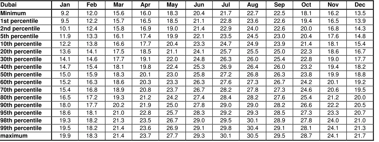
Table A.3 Wet Bulb Distribution for Dubai (oC) for January through December ... 66
Table A.4 Wet Bulb Distribution for Doha (oC) for May through October... 67
Table A.5 Wet Bulb Distribution for Bahrain (oC) for January through December ... 68
Table A.6 Wet Bulb Distribution for Dhahran (oC) for January through December... 69
Table A.7 Wet Bulb Distribution for Kuwait (oC) for January through December... 70
Table A.8 Wet Bulb Distribution for Jeddah (oC) for January through December... 71
Table A.9 Wet Bulb Distribution for Aqaba (oC) for January through December ... 72
Table A.10 Wet Bulb Distribution for Adabiya (oC) for January through December ... 73
Table C. 1.1 Distribution of Heat and Water Vapour Sources Within Cattle CFD Model... 88
Executive Summary
This final report documents the data analysis, mathematical modeling and software development of ‘HS’, a program to estimate the risk of mortality due to heat stress in livestock decks on voyages from Australia to the Middle East. The report now includes the risk management model for open decks which is also fully implemented in the software. The software has been expanded and revised following industry workshops and is now released as “HS Version 2.1”.
The risk assessment method takes account of weather at destination and en route, animal acclimatisation, coat and condition and the ventilation characteristics of the ships.
Very little solid information is available to assist the assessment of animal mortality limits. The available data have been used to extrapolate to other animals using scaling based on dimensional analysis and knowledge of heat transfer behaviour. The weather data are also uncertain to some extent and we have decreased the observing ships’ wet bulb data probability distributions by 1oC to allow for known data deficiencies which cannot be fully corrected. With adjustments so made, it is felt that the risk predictions for voyages are neither overly conservative nor overly optimistic. This is confirmed by a new validation based on analysis of voyage 20 of the Al Shuwaikh. Certainly, high risk voyages will be identified and prevented in the future. There will always be some grey areas in estimating lower level risks around the level of the target risk limit.
Further animal house work and voyage weather and animal observations will allow the input data to be improved with time, possibly resulting in adjustments to the model. It is suggested that the model, the software and the outcomes be reviewed annually following the northern summer.
There is little recorded information on the temporal variation of wind in discharge ports. For this reason, the proposed method for control of heat stress risk on open decks is different to that for closed decks. For open decks we recommend that:
Open decks on new ships should be ventilated and assessed as for closed decks
Existing ships with mechanical PAT on open decks of less than 150m/hr should undertake engineering investigations to identify all reasonably practical measures for improving PAT.
1 Introduction
1.1 Background
High mortality incidents in livestock export to the Middle East over the 2002 northern summer have highlighted systemic weaknesses in the standards and procedures previously applied to animal welfare and mortality risk reduction on such voyages. There has been a need to bring practices into line with the current risk management knowledge which has been documented particularly over the last two years.
From work for LiveCorp/MLA by Dr Richard Norris of AgWA, it is known that the three principal causes of mortality in sheep and goats are inanition (failure to eat), feedlot related salmonellosis and heat stroke. Inanition causes weaknesses which predispose the animal to other diseases (including salmonellosis) and is characterised by a trickle of mortality which, if anything, builds slightly towards the end of long haul voyages. Feedlot related salmonellosis is evidenced by scour, and mortalities generally peak within the first 5 days of a voyage and subside to inanition type levels later in the voyage, when the two diseases are often likely to be in combination anyway. When either of these problems is very severe, the combination of the two may push the mortality rate above the 2% reporting threshold.
Heat stroke, and the precursor heat stress, occurs as sudden deck-wide epidemics when the environmental conditions are such that animals cannot reject sufficient heat to maintain core body temperature at normal levels in the face of the ongoing generation of internal body (metabolic) heat. Before a major epidemic becomes apparent, increasing environmental heat will drive up mortality rates as those sheep weakened by salmonellosis or other diseases succumb before the general population. Oddly, some degree of inanition may assist survival in a heat wave by decreasing the animals’ internal heat generation. This is not yet certain.
For cattle, the principal causes of mortality are trauma, respiratory disease and heat stroke. Trauma is minimised through animal housing design and handling procedures. Respiratory disease prevention is the subject of a current LiveCorp/MLA study led by Dr Simon More. Heat stroke and heat stress in cattle follow epidemiological patterns similar to those for sheep, albeit with onset over a wide range of conditions for different livestock types and lines.
Studies coordinated by LiveCorp and MLA and managed principally by Dr Conrad Stacey of Maunsell Australia and Dr Simon More of AusVet Animal Health Services have elucidated and documented the science relating to the heat stress, ventilation and salmonellosis issues relevant to livestock export by sea.
1.2
Scope and Objectives
This project focussed on the risk of stress and mortality caused by heat. The risk of heat stress relates to parameters in three broad categories:
Weather
Animal physiology Ship ventilation
can be justified by both the knowledge of risk factor interactions and the confidence level in relevant parameters.
The principal outputs of the project are, for sheep and cattle voyages to the Middle East:
A clear and transparent method of risk evaluation Documented risk parameters
A simple software tool to assist exporters with heat stress risk assessment
1.3 Project
Progress
Project LIVE.116 is now complete except for the software maintenance period. HS Software has been revised to Version 2.1.
1.4
A Quick Look at Outcomes
The purpose of the risk estimate software is to automate the calculation process involving table look-ups and repetitive calculations for many combinations of input variables. To assist in understanding the outcomes, Figure 1.1, Figure 1.2 and Figure 1.3 show the closed deck data in a different form. They give allowable stocking density as a fraction of the LEAP maxima for three common classes of animal.
Since very few cattle decks have a pen air turnover (PAT) of 100m/hr or less, Figure 1.1 effectively shows that the current fleet can transport northern Australia Bos indicus animals with relative safety all year round. This accords with industry experience. Figure 1.2 shows that, unlike Bos indicus, Bos taurus animals will require light stocking for much of the year and should really not be delivered in August. Figure 1.3, for 40kg Merinos, looks similar to Figure 1.1 for 300kg Bos indicus, however it has more serious implications as many sheep decks have a PAT less than 100m/hr.
Figure 1.1 Allowable Stocking Fraction for 300kg Bos indicus, fat score 3,
acclimatised to 15oC wet bulb
0% 10% 20% 30% 40% 50% 60% 70% 80% 90% 100% J anuar y F ebr uar y Ma rc h Ap ri l Ma y J une Ju ly A ugus t S ept e m ber O c tober N ov e m ber D ec e m ber St o c k ing f rac ti on
PAT 50 m/hr PAT 70 m/hr PAT 100 m/hr PAT 150 m/hr PAT 200 m/hr PAT 250 m/hr
South to Gulf, Bos indicus 300kg, fat score 3, only one type coat, 15degC wb acc., <2% chance of 5%mortality.
Figure 1.2 Allowable Stocking Fraction for 300kg Bos taurus, fat score 3, acclimatised
to 15oC wet bulb, mid season coat
0% 10% 20% 30% 40% 50% 60% 70% 80% 90% 100% J a nu ar y Feb rua ry Ma rc h Ap ri l Ma y Ju n e Ju ly Au g u s t S e pt em be r Oc to b e r No v e m b e r De c e m b e r S tock ing f ra c ti on
PAT 50 m/hr PAT 70 m/hr PAT 100 m/hr PAT 150 m/hr PAT 200 m/hr PAT 250 m/hr
Figure 1.3 Allowable Stocking Fraction for 40kg Adult Merinos, fat score 3,
acclimatised to 15oC wet bulb, shorn
0% 10% 20% 30% 40% 50% 60% 70% 80% 90% 100% J anuar y F ebr uar y Ma rc h Ap ri l Ma y J une Ju ly A ugus t S ept em be r Oc to b e r N ov em ber De c e m b e r St oc k ing f ra c ti o n
PAT 50 m/hr PAT 70 m/hr PAT 100 m/hr PAT 150 m/hr PAT 200 m/hr PAT 250 m/hr
South to Gulf, Merino adult 40kg, fat score 3, shorn coat, 15degC wb acc., <2% chance of 5%mortality.
1.5
Recommendations for Further Work
Following the principal risk influences, further work could focus on weather, animal parameters or ship ventilation.
1.5.1 Weather
It is considered that the best use has already been made of available data. A serious weather monitoring program would take decades to build statistically useful data to supplant the data already available. However, monitoring Gulf and Red Sea weather has a distinct advantage in being able to corroborate shipboard measurements whenever an incident is being investigated. For example; satellite based weather data could assist in assessing heat stress effects on the Cormo Express voyage turned away from Saudi Arabia.
1.5.2 Animal
Parameters
While the animal heat stress thresholds (HST) and mortality limits (ML) are uncertain, the trends of there parameters with the risk influences of weight, breed, coat, acclimatisation and fat score are less clear.
It may well be that, for example, lambs could be loaded more densely than suggested, with the heaviest wethers requiring still more space. We believe that the targets for hot house research work (in order of priority) are:
Influence of weight on the HST of sheep Influence of weight on the HST of cattle HST of crossbred vs. Merino sheep Influence of Bos indicus infusion on HST
Influence of acclimatisation on the HST of sheep and cattle Influence of fat score on the HST of sheep and cattle
1.5.3 Vessel
Ventilation
HS Version 2.1 has no allowance for air jetting or variation of ventilation along a deck. More importantly, the vessel ventilation data in HS Version 2.1 remain largely unaudited. We recommend that all vessels on the trade be subject to ventilation surveys to verify or amend PAT data which are central to risk assessment.
Jetting assessment is more problematic. We now take the view that the air flows to give the necessary pen air turnover will be sufficient to give effective jetting (and general circulation) over animal areas. Lack of jetting will be correlated with low PAT. If the input risk data are (appropriately) taken as relevant to pens with jetting, then the method may only be criticised for not applying a ‘de-rating’ to areas with no jetting and only a general drift velocity. Such a de-rating could be included later if required as provision has been made in the software data structure.
2 Weather
The key weather influences on the live export trade, notably the detailed seasonal variations of wet bulb temperature climatologies, are described in the following sections. Section 2.1 focuses on the weather experienced in the nine key Middle Eastern ports of disembarkation. Section 2.2 looks at the voyage weather covering the oceanic areas ranging from the Persian Gulf and Gulf of Oman, the Red Sea and Gulf of Aden, the Arabian Sea and the Indian Ocean. Section 2.4 provides an overview of the wet bulb climatology of the Australian ports of departure.
2.1
Middle East Weather
2.1.1
Data Sources and Quality
2.1.2
General Temperature Observations
Northern Winter
The six month period from November to April marks the coolest six months of the year for the Middle East ports used for the livestock trade from Australia. As is the case for most desert climates, these ports can and do experience periods of quite cool weather. However, they do not reach the extremes of cold experienced in more northern climates and across southern Australia during the southern winter. This is due to the moderating effects of the Persian Gulf, Red Sea and Gulfs of Aqaba and Oman. The sea temperatures in these seas do not drop as rapidly as do the temperatures over land, which have been known to drop as low as –9C inland from Kuwait. In general the sea surface temperatures stay in the mid to high 20s.
Temperatures, humidities and wet bulb temperatures drop rapidly during the months of October and November from their summer maxima then tend to stabilize from December through until March when they start to rise again. Short-lived hot spells are possible during the months of November and April, particularly at the southern most ports and Jeddah. Dust storms are also relatively common during these months.
Although still very dry by Australian standards, a few weather systems during this season bring short-lived periods of rain. This is more so in the northern ports of Aqaba, Adabiya and Kuwait. Most ports would experience fewer than 10 wet days (days on which more than 0.2mm of rain is reported) for the entire winter period.
Northern Summer
The heat and humidity levels rapidly build across all Middle East ports during the period from May through to June. First affected are the southern most ports of Muscat and Fujairah where the sun rapidly climbs to almost overhead during May. The heat and humidity extend northwards with central Gulf ports from Dubai to Doha, Bahrain and Dhahran becoming consistently hot and humid from June onwards. Jeddah, on the Red Sea, also enters its' very hot season in June. The true peak of heat and humidity sets in for the northern most ports of Kuwait in the Gulf and Aqaba in the Red Sea (Gulf of Aqaba) towards the end of June into early July. The high heat and humidity levels continue through until the end of September, except for the southern Persian Gulf ports where the high humidity levels linger into October. October is a transition month with shorter spells of hot and humid weather becoming interspersed with cooler and drier conditions. In general, lower humidities tend to be experienced when there are stronger winds, particularly from the NNW (the “Shamal as it is known in the Persian Gulf) or when there are lighter offshore winds from the nearby desert. The latter are often associated with stronger winds, as the sea breeze will tend to overpower any lighter offshore breeze.
Detailed descriptions of the climatology for each discharge port are given in Appendix A.
2.2 Voyage
Weather
While the weather in the Middle East was understood to dominate the heat stress risk for much of the year, it was important to verify that understanding with hard data, and to check the importance of conditions en route to heat stress risk during the northern winter. Both of these were done using data from the Voluntary Observing Ships programme.
still data included in this dataset that was considered to be potentially erroneous, particularly at the high end of the wet bulb temperature distribution. To identify and completely remove all of these incorrect data is a large task and one outside the scope of this project. However, to compensate at least partially for these incorrect data, monthly Normal wet bulb temperature distributions were manually derived in the highest oceanic sector for each of the four Middle East routes.
The oceanic regions were subdivided into approximately 30 separate zones for ease of analysis. The Persian Gulf was divided into 4 zones representing the northern, central and southern regions of the Gulf plus the Gulf of Oman. The Red Sea was subdivided into four latitudinal zones in an attempt to better quantify the north – south wet bulb gradients within this elongated sea with some extra detail around the Straits of Mandeb that separates the Red Sea from the Gulf of Aden. The open oceanic zones were generally five degree latitude and 10 degree longitude boxes, increasing to ten degree square latitude / longitude boxes south of 10oS where the wet bulb regime was considered more benign.
The north of the Persian Gulf exhibits the greatest seasonal variations in wet bulb distribution of all the regions included in this study. The combination of shallow waters to the north of the Gulf combined with its northern most location is the reason for this large wet bulb range. During half of the year the wet bulb rarely approaches 26oC. However, during the months of June to September the mean wet bulb temperature exceeds 26oC and peaks around 33oC in late July to early August. The central and southern parts of the Persian Gulf are also subject to strong seasonal variations, although not as large as in the north. Once again it is the four months from June to September inclusive when the mean wet bulb temperature exceeds 26oC. The highest wet bulb temperatures are recorded in August when the mean rises to 29oC and maximum values are known to exceed 33oC. These values, recorded over the western approaches to the Straits of Hormuz, are the highest of any region included in this study.
The eastern approaches to the Straits of Hormuz have a longer period of elevated wet bulb temperature – with the period when the mean wet bulb temperature exceeds 26oC lasting from May through until towards the end of September, when the wet bulb temperature drops rapidly. The highest mean wet bulb is reached relatively early in the summer in June and July when the wet bulb averages 28.7oC. The strengthening SW monsoon through the Arabian Sea helps to drop the wet bulb slightly in this region in August and particularly in September.
The Gulf of Aden region is interesting in the fact that its humidity peaks earlier than all other parts of the Middle East Oceans – reaching a mean value of 27.7oC in June with the 98th percentile reaching 31oC. Wet bulb temperatures remain above 26oC on average from May through until September but the extent of the rise is limited by the development of the low level Somali jet that affects the waters in the entrance to the Gulf of Aden. There is a late secondary peak in humidity in this region in September when the Somali jet dies away before the seasonal cooling sets in during October.
The open oceanic waters of the Indian Ocean are characterised by generally lower mean wet bulb temperatures than experienced in the Persian Gulf and the Red Sea, as well as the Gulfs of Oman and Aden. However, there are times of the year when there can be sizeable areas with raised wet bulb temperatures. The region between 15oN and 10oN from 50oE to 70oE experiences a period from May to June when the mean wet bulb temperature exceeds 26oC – peaking at 26.7oC in June. The 98th percentile reaches 30oC in June. This is the time of northward transit of the sun and it coincides with prolonged periods of light wind conditions. The May to June period is also very humid over the approaches to the Gulf of Oman, although wet bulb temperatures are generally not quite as high as in the regions immediately to the south and west. The region between 5oN and 10oN between 70oE and 80oE to the west of the southern tip of India also warrants a mention. This region experiences mean wet bulb temperatures above 26oC early in the season – during April and May – as the sun traverses overhead and reaches 29oC on 2% of occasions.
The near equatorial region – from 5oN to 5oS is characterised by a relatively uniform wet bulb temperature distribution – mostly around 25oC to 26oC. There is a slight peak in the period from April to June as the southeast trade winds tend to be weaker at this time of the year and the SW monsoon is yet to develop. It is notable that although there is a strong tendency for most wet bulb temperature to fall within the 25 to 26oC range there are quite a few periods of time when the wet bulb temperature reaches 28oC. Although they are scattered throughout the year there is a preference for them to occur in June. They tend to coincide with periods of time when the SE trade winds are weak and there are large areas of light winds lasting several days. The voyage of the Becrux encountered one such period of elevated wet bulb temperature – reaching 28oC in Late June 2002. It is possible to avoid these areas on most occasions by changing the route to stay over regions where the wind is stronger, although this is not a practice currently followed.
South of 5oS there are periods of time between March and May when the mean wet bulb temperature is elevated close to 26oC. In April the wet bulb temperature reaches 28oC on 10% of occasions and there are occurrences in other months of the year when the temperatures reach 28oC.
South of 10oS there is not great concern about oceanic wet bulb temperatures. Trade winds keep the ocean surface well mixed and as a result wet bulb temperatures rarely exceed 26oC.
2.2.1
Data Source and Quality
Data for the voyage analysis were purchased from the ‘National Climatic Data Center’ (a US government body), covering the ocean areas of interest for the last 10 years.
The most likely error in reporting wet bulb temperature is that the wet bulb itself becomes dry or does not have air freely circulating around it. Both problems increase the reported wet bulb temperature. It was felt, after analysis, that the oceanic data had a significant fraction of ‘over-estimated’ wet bulb values, making a difference to the statistics at the high temperature end of the range. For each of the ocean zones, this has been manually accounted for when fitting Normal distributions to the data. When doing this in Gulf and Red Sea areas, acknowledgement was also made of the statistics of the more reliable data from adjacent ports. This calibration against the shore data led to a blanket reduction in the mean by 1oC being applied to all ship sourced wet bulb statistics. Thus, the data in Table 2.1 may appear to be 1oC too cool if compared only to the NCDC data, however they are now consistent with the shore based records.
2.3
Use of Voyage and Destination Weather
Each of the zones had sufficient data (>1000 points/month) to generate a realistic probability distribution of wet bulb temperature within the zone for each month. The least populous zones were 10oS to 15oS where conditions are milder. Those zones clearly do not control the heat stress risk of voyages to the Middle East and so the sparsity of data is not an issue. Appendix A tabulates the wet bulb temperature probability distributions derived from the NCDC data set. As discussed in Section 2.2.1, these data were combined into voyage maxima for each month along each of 4 routes; northern Australia to the Gulf, northern Australia to the Red Sea, southern Australia to the Gulf and southern Australia to the Red Sea. Normal distributions were adjusted to fit the worst case probabilities for each route and month (48 cases) applying meteorological judgement in allowing for the known data deficiencies. In fitting Normal distributions to the wet bulb data, attention was only paid to the top 50% of the distribution. This may give an error at lower temperatures however low temperatures are not relevant to heat stress. The resulting 48 pairs of mean and standard deviation are given in Table 2.1. Note that, in order to improve agreement with shore based data, and acknowledging known data deficiencies, the risk estimation currently applies a 1oC shift to all means. This adjustment is already included in Table 2.1.
Table 2.1 Idealized “Normal” Wet Bulb Probability Distributions (mean ± standard deviation)
Month North to Red Sea South to Red Sea North to Gulf South to Gulf
January 24.2 ± 1.30 24.0 ± 1.30 24.1 ± 1.40 24.0 ± 1.40 February 24.4 ± 1.40 24.2 ± 1.30 24.4 ± 1.40 24.2 ± 1.35 March 24.6 ± 1.35 24.5 ± 1.40 24.6 ± 1.35 24.5 ± 1.30 April 25.0 ± 1.45 24.9 ± 1.30 24.9 ± 1.50 24.9 ± 1.30 May 26.3 ± 1.30 26.2 ± 1.40 25.9 ± 1.70 25.9 ± 1.70 June 27.1 ± 1.30 27.1 ± 1.30 27.4 ± 1.70 27.4 ± 1.70 July 27.4 ± 1.55 27.4 ± 1.55 28.1 ± 1.50 28.1 ± 1.50 August 27.3 ± 1.55 27.3 ± 1.55 28.2 ± 1.65 28.2 ± 1.80 September 27.1 ± 1.40 27.1 ± 1.40 27.2 ± 1.80 27.2 ± 1.70 October 25.8 ± 1.50 25.8 ± 1.50 24.7 ± 1.90 24.7 ± 1.90 November 24.0 ± 1.35 24.0 ± 1.35 24.1 ± 1.45 24.1 ± 1.45 December 24.0 ± 1.25 24.0 ± 1.25 24.1 ± 1.25 24.0 ± 1.25
2.4 Departure
Ports
Wet bulb data for all significant departure ports have been sourced and analysed. The detailed port information given below has now been largely superseded by a change in the modelling of acclimatisation which followed from discussions at the Milestone 2 meeting in Canberra. The acclimatisation factor, which is discussed in detail in Section 3.3.2, is now based on ‘acclimatisation zones’. Across any one acclimatisation zone, the wet bulb variation through the year is reasonably consistent. These zones were selected using summary wet bulb data not only from the ports but from a total of 97 weather stations across Australia. Figure 2.2 shows the draft acclimatisation zone map with the weather sites marked. The numbers next to each site show the approximate average wet bulb temperatures for January (top number) and July (bottom number). Figure 2.3 is the zone map included in the software.
Where the animals are transported from the property of origin to the ship and spend only a day or two near the port, it is clear that the acclimatisation zone entered should be appropriate to the property of origin. Similarly, if the animals have spent considerable time at the port (say 15 days or more) they may be considered as being acclimatised to the port conditions and the zone entered into the software should be that of the port. To cover the grey area in between these two, we suggest the following approach.
If the animals spend less than 4 days between the property of origin and sailing, the zone is taken at the property of origin.
If the animals spend 15 days or more in the zone of the port, then the appropriate zone is that covering the port.
If the animals spend between 4 and 14 days in the port zone, the zone number entered should be the average of the zone numbers for the property of origin and the port (rounded down to the nearest integer if required).
Arguments could be mounted for a different approach for special cases. For example, cattle sourced in zone 3, spelled for 8 days in zone 1 and held for 4 days near the zone 2 port would have uncertain acclimatisation. The number chosen is a matter for judgment on each occasion.
Table 2.2 gives the adopted wet bulb temperatures for acclimatisation for each month and zone. The same data are shown graphically in Figure 2.4
Table 2.2 Acclimatisation Wet Bulb Temperatures by Zone and Month ZONE
1 2 3 4 5 6
Jan 15 17 19 21 23 25
Feb 14.5 16.5 18.4 20.4 22.3 24.3 Mar 13 15 16.8 18.6 20.5 22.3 Apr 11 13 14.5 16.3 18 19.5 May 9 11 12.3 13.9 15.5 16.8 Jun 7.5 9.5 10.6 12.1 13.7 14.7
Jul 7 9 10 11.5 13 14
Aug 7.5 9.5 10.6 12.1 13.7 14.7 Sep 9 11 12.3 13.9 15.5 16.8 Oct 11 13 14.5 16.3 18 19.5 Nov 13 15 16.8 18.6 20.5 22.3 Dec 14.5 16.5 18.4 20.4 22.3 24.3
Figure 2.4 Acclimatisation Wet Bulb Temperatures by Zone and Month 6 8 10 12 14 16 18 20 22 24 26 Ja n Fe b Ma r Ap r Ma y Ju n Ju l Au g Se p Oc t No v De c Ja n A c c lima tis a tio n w e t b u lb t e mp . ( C ) Zone 1 Zone 2 Zone 3 Zone 4 Zone 5 Zone 6
3 Animal
Parameters
The overall model for heat stress risk is reliant on a sound understanding of four components relating to animal heat tolerance, including:
An evaluation of the heat stress threshold (HST) and mortality limit (ML) in sheep and cattle from available experimental and observational data for different breeds.
An assessment of the principal modifiers of HST and ML including acclimatisation, weight/age, body condition and wool/coat length.
Thermal modelling and scaling parameters to allow interpolation and extrapolation of recorded data to cover the range of animal parameters, and to correlate the available data into a single coherent set.
The statistical variability of heat tolerance within animal populations.
Detailed information on source data is presented in Appendix B.
3.1
Appropriate Terminology and Definitions
The issues of terminology and definition have been discussed at length in several forums recently. There is often confusion and sometimes disagreement about the definition and use of measures relating to heat stress in animals. We have undertaken a detailed review of relevant literature to capture current international thinking and ensure that the terminology does not conflict with international best-practice in this area. Detailed background on this is given in Appendix B.
The upper critical temperature (UCT) is a common term in the literature, used to describe the dry bulb temperature at the upper boundary of the thermoneutral zone. Unfortunately UCT as defined cannot exist unless heat stress is closely related to dry bulb temperature. In the project proposal we suggested an Upper Critical wet bulb Temperature (UCwbT) to recognise that heat stress is more closely related to wet bulb temperature. A recent industry meeting in Canberra agreed that UCwbT was too much of a mouthful and, by consensus, adopted the term Heat Stress Threshold (HST). On balance and suitable to the requirements of industry and this model, we believe that HST should be defined as ‘the maximum ambient wet bulb temperature at which heat balance of the deep body temperature can be controlled using available mechanisms of heat loss’.
That is; when the local air wet bulb temperature reaches any animal’s HST, the animal is on the verge of becoming stressed. As implied above, incipient stress in this sense means the first uncontrolled rise in core body temperature. We take this as being 0.5oC above what the core temperature would otherwise have been.
The same meeting in Canberra agreed ‘Mortality Threshold’ as the descriptor of the wet bulb temperature at which an animal will die. In this context, ‘threshold’ is perhaps inappropriate as it implies that the animal has started dying and might finish dying at another temperature. We prefer ‘Mortality Limit’ or ML as the limiting wet bulb temperature above which the animal is dead.
3.2
Evaluating the Heat Stress Threshold and Mortality
Limit
A review has been made of data on the HST and ML of cattle and sheep during live export. A range of information sources were used, including:
Published information (from scientific literature)
Experimental information (particularly LiveCorp-funded R&D projects SBMR.002, LIVE.209 and LIVE.212)
Voyage investigation (Voyage 1 of the MV Becrux)
Evaluation of these parameters is in two stages. First, the parameters specific to each case have to be assessed from the given data. Then, the understanding of all the modifying influences (weight, acclimatisation, coat and condition) is used to link the assessed ‘raw’ parameters into a cohesive framework, allowing the HST and ML to be estimated for any new animal with its own combination of modifying factors.
Because there may be deficiencies associated with each data source, it is important to simultaneously consider all of these results in the evaluations of HST and ML in sheep and in cattle. For studies with populous data sets, a form of multi-variate regression would normally be applied to estimate the factors. This is simply not possible with the present limited data set and so the fitting of factors to raw data has been done manually.
DATA SET ACCLIMATISATION WB TEMP WEIGHT (KG) COAT FAT SCORE F acc Fwe ight Fc oa t Fc ond
HST ML
HST diff ML diff
MLdiff / HSTdiff
REFERENCE
BOS TAURUS TABLE
Becrux soft southern cattle 12 350 winter 5 1.057 1.05 1.1 1.2 26.0 30.0 14.0 10.0 0.71 Inferred base, 350kg 15 350 mid 3 0.995 1.02 1 1 30.0 32.9 9.99 7.13 0.71 Inferred base, 300kg 15 300 mid 3 0.995 1 1 1 30.5 33.2 9.49 6.78 0.71 1
Inferred, 350kg,summer 18 350 summer 3 0.934 1.05 0.93 1 31.3 33.8 8.72 6.23 0.71
Ausvet report. ML looks OK.
HST based only on first report of stress.
Murdoch Angus animals 15 370 mid 3 0.995 1.07 1 1 28.0 33.0 12.0 7.0 0.58 Inferred base, 300kg 15 300 mid 3 0.995 1 1 1 28.8 33.5 11.2 6.53 0.58 2
Inferred, 300kg,summer 15 300 summer 3 0.995 1 0.93 1 29.6 33.9 10.4 6.07 0.58
Murdoch 'experiment 1'
ML is 1.0 deg above point where mortality seemed likely soon Murdoch Murray Grey X 13 340 mid 3 1.036 1.04 1 1 29.0 33.0 11.0 7.0 0.64
inferred base, 300kg 15 300 mid 3 0.995 1 1 1 29.9 33.5 10.1 6.45 0.64 3
inferred, 300kg,summer 15 300 summer 3 0.995 1 0.93 1 30.6 34.0 9.43 6.0 0.64
Murdoch 'experiment 2'
ML is 0.5 deg above point where mortality seemed likely soon Friesan 12 200 mid 3 1.057 0.87 1 1 29.0 33.4 11.0 0.6
7
inferred base, 300kg 15 300 mid 3 0.995 1 1 1 28.2 32.9 11.8 0.6
SBMR.002, voyage 5, D4,P35.
Euro cross bull calves 12 200 mid 3 1.057 0.87 1 1 31.0 34.6 9.0 0.6 8
inferred base, 300kg 15 300 mid 3 0.995 1 1 1 30.3 34.2 9.69 0.6
SBMR.002, voyage 5, D5,P5,P19,P29&P37.
Southern bulls 12 385 mid 3 1.057 1.09 1 1 29.5 33.7 10.5 0.6 9
inferred base, 300kg 15 300 mid 3 0.995 1 1 1 30.9 34.5 9.11 0.6
SBMR.002, voyage 5, D3,P7&P47.
BOS INDICUS TABLE
Acclimatised, Darwin, 420kg 23 420 n/a 3 0.831 1.12 1 1 32.5 36.0 7.5 4 0.53 inferred base 420kg 15 420 n/a 3 0.995 1.12 1 1 31.0 35.2 8.98 4.79 0.53 6
inferred base 300kg 15 300 n/a 3 0.995 1 1 1 32.0 35.7 8.04 4.29 0.53
guess from SBMR.002, voyage 4. ML taken above all wb noted (no mort.)
Unacclimatised, TSV, 420kg 12 420 n/a 3 1.057 1.12 1 1 30.5 35.5 9.5 4.5 0.47 inferred base 420kg 15 420 n/a 3 0.995 1.12 1 1 31.1 35.5 8.95 0.5 5
inferred base 300kg 15 300 n/a 3 0.995 1 1 1 32.0 36.0 8.01 0.5
SBMR.002, voyage 3, guess
Murdoch Bos indicus 12 350 n/a 3 1.057 1.05 1 1 32.5 36.0 7.5 4 0.53 inferred base 350kg 15 350 n/a 3 0.995 1.05 1 1 32.9 36.2 7.06 0.53 4
inferred base 300kg 15 300 n/a 3 0.995 1 1 1 33.3 36.4 6.71 0.53
DATA SET
ACCLIMATISATION
WB TEMP
WEIGHT (KG)
COAT
FAT SCORE
F
acc
Fwe
ight
Fc
oa
t
Fc
ond
HST ML
HST diff ML diff
MLdiff / HSTdiff REFERENCE
MERINO TABLE
Voyage 1 adults 12 52 shorn 3 1.057 1.01 1 1 29.5 35.0 10.5 5 0.48 10
inferred base, 40kg 15 40 shorn 3 0.995 0.96 1 1 30.6 35.53 9.38 4.47 0.48
Live.212 v1, lower mort.~32
Voyage 1 woolly ewes 12 54 woolly 3 1.057 1.02 1.12 1 28 34.29 12 0.48 11
inferred base, 40kg 15 40 shorn 3 0.995 0.96 1 1 30.5 35.47 9.5 0.48
Live.212 v1 D8, P30
Voyage 1 lambs 12 38 shorn 3 1.057 0.95 1 1 26 35.0 14 5 0.36 12
inferred base, 40kg 15 40 shorn 3 0.995 0.96 1 1 26.7 35.24 13.3 4.76 0.36
Live.212 v1, D5, P1&2
Voyage 2 adults 11 60 shorn 3 1.077 1.04 1 1 29.5 35.0 10.5 0.48 13
inferred base, 40kg 15 40 shorn 3 0.995 0.96 1 1 31.1 35.74 8.94 0.48
Live.212 v2, lower mort.~32.5
AWASSI TABLE
Voyage 1 lambs 12 38 hairy 3 1.057 0.95 1 1 28 35.71 12 0.36 14
inferred base, 40kg 15 40 hairy 3 0.995 0.96 1 1 28.6 35.92 11.4 0.36
Factor Bos taurus Bos indicus Sheep
Base Weight (kg) 300 300 50
Weight Index n 0.33 0.33 0.2
Core Temperature (oC) 40 40 40
Fat Score 0 9 9 9
Fat Score 1 0.9 0.9 0.9
Fat Score 2 0.95 0.95 0.95
Fat Score 3 1 1 1
Fat Score 4 1.1 1.07 1.07
F Condition
Fat Score 5 1.2 1.2 1.2
Mid 1 -
-Summer (shiny) 0.93 - -
Winter (hairy) 1.1 - -
Normal - 1
-Hairy (Awassi only) - - 1
Mid (10 to 25mm) - - 1.08
Shorn (under 10mm) - - 1
F Coat
Woolly (over 25mm) - - 1.12
Fully Acclimatised 0.79 0.79 0.79
Fully Unacclimatised 1.26 1.26 1.26 F Acclimatisation
Slope -0.0235 (per degree) -0.0235 (per degree) -0.0235 (per degree)
Fully Acclimatised 25 25 25
Twb Break
Table 3.4 Base Heat Stress Threshold and Mortality Limit Values for the ‘Standard’ Animals
Bos taurus Bos indicus Merino Awassi
Base Parameter beef dairy beef 25% indicus
50% indicus
adult lamb adult lamb
Weight (kg) 300 300 300 300 300 40 40 40 40
Core Temperature (degrees C) 40 40 40 40 40 40 40 40 40
Condition (Fat Score) 3 3 3 3 3 3 3 3 3
Coat mid mid N/A N/A N/A shorn shorn hairy hairy
Acclimatisation WB Temp 15 15 15 15 16 15 15 15 15
Base HST (degrees C) 30 28.2 32.5 31.25 31.875 30.6 26.7 31.9 28.6
Base ML (degrees C) 33.2 32.9 36.0 34.60 35.30 35.5 35.20 36.1 35.90
Beta distribution lower limit (degrees C) 30.31 29.88 34.30 32.30 32.30 33.58 33.17 34.52 34.15
It is particularly difficult to get good data on mortality limits. It is not possible to kill large numbers of animals in the lab and, when significant mortality occurs at sea, the crew are understandably more concerned with managing the situation than making careful records of the weather and pen environments. For Bos taurus, voyage 1 of the Becrux gave some data and we have also used the opinion of the Murdoch University team that their Bos taurus animals were close to the limit when conditions were finally relieved. For Bos indicus, no data are available. Taking a mortality limit above the highest temperature at which animals were monitored does not give an accurate figure. Nevertheless, an estimate has been made. It can be revised at any time in the future as new data are examined.
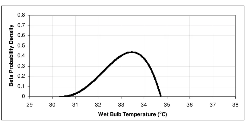
We don’t expect that we will ever see data which show mortality as a function of wet bulb temperature for a large group of one type of animal. Accordingly, we have had to synthesise the probability distributions of HST and ML. Appropriate to the nature of the problem, we chose a skewed beta distribution. This has the property that a small number of animals respond at lower temperatures but the distribution is more compressed above the 50 percentile. That is; no animals survive at wet bulb temperatures just a little above the temperatures that will kill half their number, whereas there are animals which are significantly ‘softer’ than most. In selecting the beta distributions, greater attention has been paid to the low temperature end. The top end of the distribution is really only of academic interest as a 50% mortality rate is already a major problem and so arguments over prediction of 60% versus 75% mortality are not useful.
[image:30.595.143.549.430.631.2]The beta function probability distributions of mortality limit for key classes of animal are shown in Figure 3.1, Figure 3.2, Figure 3.3, Figure 3.4, Figure 3.5, Figure 3.6, Figure 3.7, Figure 3.8 and Figure 3.9.
Figure 3.1 Beta Function Probability Distribution – Bos taurus - beef
0 0.1 0.2 0.3 0.4 0.5 0.6 0.7 0.8
29 30 31 32 33 34 35 36 37 38
Wet Bulb Temperature (oC)
B
e
ta
P
ro
ba
bil
it
y
D
e
ns
it
Figure 3.2 Beta Function Probability Distribution – Bos taurus - dairy 0 0.1 0.2 0.3 0.4 0.5 0.6 0.7 0.8
29 30 31 32 33 34 35 36 37 38
Wet Bulb Temperature (oC)
B e ta P rob a b il it y D e n s it y
Figure 3.3 Beta Function Probability Distribution – Bos indicus
0 0.1 0.2 0.3 0.4 0.5 0.6 0.7 0.8
29 30 31 32 33 34 35 36 37 38
Wet Bulb Temperature (oC)
Figure 3.4 Beta Function Probability Distribution – 25% Bos indicus 0 0.1 0.2 0.3 0.4 0.5 0.6 0.7 0.8
29 30 31 32 33 34 35 36 37 38
Wet Bulb Temperature (oC)
B e ta P rob a b il it y D e n s it y
Figure 3.5 Beta Function Probability Distribution – 50% Bos indicus
0 0.1 0.2 0.3 0.4 0.5 0.6 0.7 0.8
29 30 31 32 33 34 35 36 37 38
Wet Bulb Temperature (oC)
Figure 3.6 Beta Function Probability Distribution – Merino - Adult 0 0.1 0.2 0.3 0.4 0.5 0.6 0.7 0.8
29 30 31 32 33 34 35 36 37 38
Wet Bulb Temperature (oC)
B e ta P rob a b il it y D e n s it y
Figure 3.7 Beta Function Probability Distribution – Merino - Lamb
0 0.1 0.2 0.3 0.4 0.5 0.6 0.7 0.8
29 30 31 32 33 34 35 36 37 38
Wet Bulb Temperature (oC)
Figure 3.8 Beta Function Probability Distribution – Awassi - Adult 0 0.1 0.2 0.3 0.4 0.5 0.6 0.7 0.8
29 30 31 32 33 34 35 36 37 38
Wet Bulb Temperature (oC)
B e ta P rob a b il it y D e n s it y
Figure 3.9 Beta Function Probability Distribution – Awassi - Lamb
0 0.1 0.2 0.3 0.4 0.5 0.6 0.7 0.8
29 30 31 32 33 34 35 36 37 38
Wet Bulb Temperature (oC)
B e ta P rob a b il it y D e n s it y
3.3
Scaling HST and ML
As mentioned in the above section, heat stress threshold and mortality limit for any given line of animal are estimated by scaling the values from those of a standard animals of the same type. The various physical characteristics (weight, acclimatisation, coat and condition) will affect the temperature difference required between the animal and its environment for rejection of metabolic heat. The factors assigned to each feature act in the model to modify this temperature difference. That is; using TCORE as the animal’s core temperature and
adjustment factors F for each characteristic:
(TCORE – HST) = FACC x FWEIGHT x FCOAT x FCONDITION x (TCORE – base HST)
and similarly for mortality limit:
As the probability beta distribution of HST and ML for any one animal type is uncertain, the scaling of the beta distribution limits with animal characteristics cannot be any more certain. Following again the principle that the difference between core and ambient wet bulb temperatures gives the controlling temperature scale, the spread of the beta distribution is adjusted in proportion to that difference. That is; ‘softer’ lines of animals, with a lower HST, will also have a wider spread of HST within the line. The shape parameters (P and Q) which determine the skewness of the beta distribution were set by judgement and have been kept constant across all animals. For the record, we have used P = 3.50 and Q = 2.00. For a 50 percentile of 35.09oC, the minimum and maximum of the beta distribution are 33oC and 36.2oC respectively. Other distributions, including those in Figure 3.1, Figure 3.2, Figure 3.3, Figure 3.6, Figure 3.7, Figure 3.8, Figure 3.7, Figure 3.8 and Figure 3.9, are scaled from this as described above.
The following sections describe the development of each adjustment factor.
3.3.1 Weight
Scaling
The initial estimate of the weight factor is based on geometry. We make the simplifying assumption that animals of one breed are geometrically similar. This gives a surface area proportional to the two-thirds power of body mass. If the rate of production of metabolic heat per unit mass is constant (a fair approximation) then obviously the heat generated is proportional to mass. Assuming further, that the coefficients of heat transfer are independent of body mass, the required minimum temperature difference between core and wet bulb temperatures goes as the one-third power of mass. That is;
∆TCRITα m⅓ (m is animal mass)
This gives the first estimate of the weight factor as
FWEIGHT =
3 1
STANDARDm
m
or, if we believe that the one-third power may not be quite right;
FWEIGHT =
n STANDARD
m
m
When an animal of a given frame puts on weight, it does not follow the geometric rules above, with surface area growing more slowly with mass than described. This has the effect of increasing the exponent n, above, beyond 0.33. Animals with lots of weight for their frame may also attract a high condition factor and so we must be careful not to ‘double count’ the weight influence in both weight factor and condition factor.
We have also not seen a strong weight influence in moderately sized (up to 60kg) sheep. For now we have settled on n = 0.33 for cattle and somewhat arbitrarily decreased this to n = 0.2 for sheep. This is discussed further in Section 3.5.2.
3.3.2 Acclimatisation
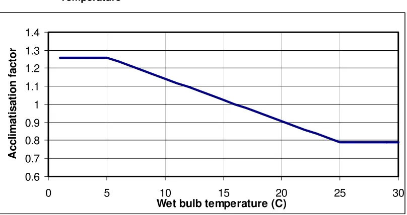
4 of the SBMR.002 cattle ship ventilation project. Voyage 3 left from Townsville with Bos indicus weighing around 420kg and acclimatised to around 12oC wet bulb. Voyage 4 left from Darwin with apparently similar animals also weighing around 420kg but acclimatised to 230C wet bulb. The difference in response between these two groups is the basis for the acclimatisation factor as plotted in Figure 3.10. The break points of the plot are also in Table 3.3.
Figure 3.10 Variation of Acclimatisation Factor with Acclimatising Wet Bulb Temperature 0.6 0.7 0.8 0.9 1 1.1 1.2 1.3 1.4
0 5 10 15 20 25 30
Wet bulb temperature (C)
A ccl im a ti sat io n f ac to r
It may well be that Bos taurus acclimatise differently, however, in the absence of solid data on this, we take the factor to be the same as for Bos indicus. It should be noted that animals with no Bos indicus infusion are hardly seen in the warmer parts of Australia and so any error in the Bos taurus acclimatisation factor is less commercially significant.
Similarly, sheep are only exported in large numbers from the southern ports and so come from a limited range of climates. An acclimatisation effect will be difficult to establish experimentally from voyages. Also because of this, errors in the factor will have a smaller impact on risk estimates. For now we have adopted the Bos indicus curve as also applying to sheep.
3.3.3 Coat
The weighting to be given to coat in the risk assessment is difficult to decide because thick coats are commonly found on cold acclimatised animals with reasonable fat scores. That is; it is difficult to separate the various effects from analysis of the available data. Of course, provided that the risk answers make sense, it is not strictly necessary to decide how much emphasis to put on coat as against condition etc. Table 3.3 shows the outcome as assessed. The ‘standard’ Bos taurus animal is assumed to have a mid season coat. No coat variation is included for Bos indicus. The standard sheep is taken as shorn, with a 12% ‘de-rating’ of woolly sheep. Awassis are assumed to come in only one variety (hairy).
3.3.4 Condition
score will also be accustomed to high fodder intakes and are likely to have a higher rate of metabolic heat generation, compounding their ‘softness’ under heat stress. Variation of response with fat score is one area where controlled environment room research is needed.
3.4 Thermal
Modelling
3.4.1 Overview
A relation between the air speed and the critical core wet bulb difference has been developed to eventually be applied to different classes of animal. The earlier heat transfer analysis has been adapted with parameters reconfigured to allow determination of the critical core wet bulb difference. The thermal model incorporates radiation, convection (forced and natural), evaporation where applicable (forced and natural) and respiratory heat rejection. These are balanced against animal metabolic rate. Heat transfer relations for a number of conditions were calculated to assess sensitivities. These sensitivities indicated where further development of the model is required.
3.4.2 Details
For a series of wet bulb temperatures, thermal equations were set up to determine the relevant heat transfer component as described below.
Radiation – this is a function of skin temperature and ambient conditions. It is assumed that the ambient dry bulb is the mean radiant temperature of the surroundings. The average skin temperature is used as the radiating temperature.
Convection – two components of convection are assessed, forced and natural. For low air velocity through the pen, natural convection will dominate. Convective heat transfer is driven by the difference between the skin temperature and ambient air temperature. It was assumed that forced convection would be relevant to a proportion of animal surface (i.e. across the animals back), while natural convection would dominate on the remainder. This seems a fair assumption as air velocities underneath and on sides of animals would be low. The bulk air movement would mostly be in the space above the animals.
Evaporation – two components of evaporation are assessed, forced and natural. As for convective heat transfer, the forced component would only act on a proportion of the animal surface.
Respiration – this is a function of breathing rate, breath air condition and ambient air condition.
Other factors such as heat storage and direct conduction to surfaces were not assessed. Heat storage effects are not significant if conditions change slowly. Conductive heat transfer would be small compared to the other heat transfer components. The above components were summed and equated to the metabolic heat generation rate. For a series of wet bulb temperatures at a given relative humidity, the equations were balanced by firstly changing the animal skin temperature and then changing the air speed across the animal. The skin temperature was allowed to rise to an upper limit of 1oC below core temperature. The air speed was then increased (if necessary) until thermal balance was achieved.
Hence, for a range of ambient wet bulb temperatures (and hence critical core wet bulb difference) the air velocity required to achieve thermal balance can be estimated. Given a known limiting critical core wet bulb difference, the required velocity to maintain appropriate heat transfer can be estimated.
3.5
Validation from a Voyage
As shown in Table 3.2, sheep mortality limit data for this project were estimated from the LIVE.212 project voyages. Since then, data from Voyage 20 of the Al Shuwaikh have become available, compiled in considerable detail. We acknowledge the active assistance of Rural Export & Trading (WA) Pty Ltd (RETWA) in compiling this information. While the data themselves are commercial in confidence, the analysis method and the pertinent conclusions are described below.
The Al Shuwaikh has both open and closed decks. Data from open decks are very difficult to analyse as even short periods of low crosswind can dramatically affect outcomes, and also the stocking data do not record which side of the deck the particular line is penned in. Mortalities on the open deck were also relatively low, making statistical treatment less reliable. For these reasons, we analysed only the closed deck data.
In assessing heat stress related mortality, the influence of other causes had to be eliminated as far as possible. An assessment was made, based on the wet bulb temperature readings, as to the stage in the voyage where heat stress was a realistic possibility. RETWA then supplied mortality data by stocking line and sailing phase, so that mortalities in the initial cooler part of the voyage could be removed from the statistics for heat stress. A heat stress mortality rate for each line was then based on the number of animals in each line which reached the hot voyage phase.
The closed deck mortality data were reduced in two ways. First, the peak recorded deck wet bulb temperatures were used to make a ‘prediction’ of the mortality for each line, for comparison with the recorded mortality. Second, a relative mortality was calculated to see whether the trend of mortality limit with weight was correctly modelled.
3.5.1
Comparison of Actual and ‘Predicted’ Mortality
The deck wet bulb temperatures were recorded to the nearest degree centigrade, presumably with an observation tolerance of ± 0.5oC. Using the methods of Section 6.1, the recorded deck wet bulb temperatures were also used to infer the ambient wet bulb temperature.
A number of lines had significantly higher or lower mortality rates than expected. Explanations for all except one prediction could be found in the data. This last under-prediction was for a line of 70kg rams from Fremantle. While the under-under-prediction is relatively minor, it suggested that the heavy rams may be less heat tolerant than the adopted heat stress model suggests.
The conclusion is that, with the uncertainties in temperature recorded, there is no inconsistency between voyage data and the ‘HS’ method given in this report, except perhaps a pointer to re-examine the mortality limits for heavy rams.
3.5.2 Relative
Mortality
The recorded mortality rate for each line was divided by the ‘expected mortality’ figure from HS to give a ‘relative mortality’. It should be remembered that the HS expected mortality figure is a statistical measure, acknowledging the weather probabilities, and does not necessarily describe an outcome for the actual voyage weather. For the present purpose, it served as a baseline from which the mortality rates of different lines were assessed relative to each other.
a stronger function of animal weight. As noted in Section 3.3.1, the exponent in the power law relating weight to weight factor for sheep was set at 0.2 on thin evidence, when geometric arguments suggested that is should be 0.33. It is recommended that this value be reviewed (and probably set closer to 0.33) at the next review of HS.
It is also noteworthy that all three of the heaviest lines on the voyage were rams. Thus, the data may include effects from both weight and testosterone. It may be that the result is due primarily to a higher metabolic rate in rams. With the present market offering almost no heavy wethers, and HS limiting the risk of future voyages, this question is unlikely to be answered by voyage results but could be addressed by controlled environment experiments on land.
4 Ship
Parameters
The data necessary for estimation of Pen Air Turnover (PAT) have been received from the owners for all of the ships on the Middle East trade.
The data have been returned to the ship owners in the form of both Excel spreadsheets and database files formatted for input into HS. The ship PAT data are variable in quality. In some instances, the data are based on ‘nameplate’ or nominal design figures, while in other cases, they are sourced from as-built measurements of the flow supplied to each deck. Nominal design figures are often lower than the actual figures as ship builders and fan suppliers allow a margin to ensure that the outcome does not fall below the specification. Because of this, a detailed survey would be likely in most cases to increase the assessed livestock loading for a given risk level.
A detailed survey would also identify any maldistribution of air between decks and avoid the associated unevenness in risk.
Since PAT is such an important parameter in assessing heat stress risk, we recommend that all ships for which HS is to be applied undergo a survey as to the flowrate and distribution of supply air.
5
Open Deck Conditions
A methodology has been developed for the Computational Fluid Dynamics (CFD) modelling of generic loaded ship decks. Three modular cases have been numerically constructed to enable simulation of single tier cattle, single tier sheep and double tier sheep decks to practically any width. Widths of 24m and 36m were nominally chosen for the study. Each single case model required over 30 hours of computation time.
These deck modules have formed the foundation for all runs performed to date which include natural convection (no ventilation from cross wind or mechanical means), mechanically ventilated, and cross wind ventilated scenarios.
The specialist software package used for the current study was Fluent from Fluent Inc., Lebanon NH, USA. This package maintains approximately 60% of the global CFD software market.
5.1 Animal
Representation
The representation of animals within the computer models incorporates the following physical effects:
Fluid blockage (blockage to the deck air flows by the animal’s presence) Energy source from skin
Energy source from breath Moisture mass source from skin Moisture mass source from breath
Momentum source from breath action at the mouth
Geometrically, each animal is represented as a prismatic object located some distance above the deck floor. Key dimensions were chosen to be representative of typical real animals (ie. height, length, overall surface area). Using such simplified prismatic bodies enables a more efficient meshing (discretisation) of the computational domain. One major issue for consideration was the space and proximity of adjacent animals. In most instances meshing would have proved much more difficult, if not impossible, if more curvilinear or ‘organic’ animal geometries had been implemented.
Numerous such geometric animal models are positioned on each modular deck tier. Pack