Ž .
Energy Economics 23 2001 211᎐226
Empirical evidence for the superiority of
non-US oil and gas investments
Jeff P. Boone
UMississippi State Uni¨ersity, P.O. Drawer EF, Mississippi State, MS 39762-5661, USA
Abstract
This paper provides empirical estimates of the return on US and non-US exploration investment. The estimates are obtained from a polynomial distributed lag model
wEconometrica 33 1965 178 that relates the present value of current period reserveŽ . x
discoveries to current and lagged US and non-US exploration investment. The empirical evidence presented in the paper indicates that the net present value of $1 invested in non-US exploration is larger in a statistically significant sense than the net present value of $1 invested in U.S exploration. In particular, results indicate that the return on non-US exploration investment is approximately 3.5 times as large as the return earned on US exploration investment. The results reported in this paper provide insights potentially useful to US energy policymakers.䊚2001 Elsevier Science B.V. All rights reserved.
Keywords:Empirical; Oil; Gas; Investments
1. Introduction
Over the past 15 years, US oil and gas firms have shifted exploration investment away from US domestic drilling to non-US drilling. During the same period, imports of oil from non-US sources have increased as a percentage of total US oil consumption. When juxtaposed, these two trends portray a troubling picture of increased vulnerability to imported oil that will likely continue for the foreseeable future.
This shift in exploration investment has been explained as a response to several
U
Tel.:q1-662-325-1634; fax:q1-662-325-1646.
Ž .
E-mail address:[email protected] J.P. Boone .
0140-9883r01r$ - see front matter䊚2001 Elsevier Science B.V. All rights reserved.
Ž .
Ž . Ž .
factors, including 1 the need to diversify exploration portfolios; 2 the opening to international investment of large, geologically attractive areas in formerly socialist
Ž .
countries; 3 the difficulty of maintaining or increasing reserve values in mature
Ž . Ž .
exploration provinces, including the United States; 4 lower ‘finding costs’; 5 Ž .
improved contracting terms with non-US governments; 6 lower foreign tax rates;
Ž . Ž
and 7 reduced US tax incentives for exploration Amoco Corporation, 1990; US Department of Energy and Energy Information Administration, 1991; Bertagne
.
1988; Wasteneys 1997 . Economic theory would suggest that exploration capital has migrated abroad because risk-adjusted returns to exploration capital invested outside the US are greater than returns earned on exploration capital invested
Ž .
inside the US Eiteman and Stonehill, 1986 . Furthermore, the desire to gain entry into non-domestic exploration provinces is thought to be a causal factor in stimulating the recent wave of mega-mergers in the petroleum industry in general ŽWeston et al., 2000 and the merger of Total and Petrofina in particular Oil and. Ž
. Gas Journal, 1998 .
Prior research has indirectly addressed the issue of whether capital migrates abroad in search of higher returns on investment by examining returns earned by shareholders, based on the assumption that higher returns on real investment will
Ž .
be reflected in higher returns to shareholders. Fatemi 1984 compares the stock returns of US multinational corporations to stock returns of US uninational corporations and concludes that both multinational and uninational corporations provide shareholders identical risk-adjusted returns, implying that returns to US real investment are the same as returns to non-US real investment. Griffian and
Ž .
Karolyi 1998 document that much of the variation in stock returns earned by shareholders in non-US oil and gas firms is attributable to a strong industry effect rather than to a strong country effect. Since one would normally expect any inter-country variation in returns to real oil and gas investment also to be reflected in a strong country effect in stock returns, these findings suggest the possibility that returns to real oil and gas investment do not differ markedly by country. In summary, the extant research provides indirect evidence that is inconsistent with the idea that exploration capital has migrated abroad in search of higher returns
Ž .
on investment. However, there is no research of which I am aware that directly tests for differences in returns to US vs. non-US exploration capital.
The purpose of this paper is to document the magnitude of the differences in returns to US exploration investment as compared to returns to non-US ex-ploration investment. In particular, I empirically estimate the net present value of oil and gas reserve discoveries per dollar invested in US exploration and compare that estimate to the estimated net present value of oil and gas reserve discoveries per dollar invested in non-US exploration. Empirical estimates of these net present
Ž .
( )
J.P. BoonerEnergy Economics 23 2001 211᎐226 213
the total present value of oil and gas reserves discovered per dollar of US exploration investment, while the sum of the discounted slope coefficients on current and lagged non-US exploration investment measures the total present value of oil and gas reserves discovered per dollar of non-US exploration invest-ment.
The empirical estimates indicate that on average, a $1 investment in US exploration activity yields over 7 years cumulative discoveries of oil and gas reserves worth $2.89 in present value, while a $1 investment in non-US exploration activity yields over 7 years cumulative discoveries of oil and gas reserves worth $10.27 in present value. Furthermore, these present values differ in a statistically significant sense. These results are consistent with the idea that US oil and gas firms have shifted exploration dollars overseas in search of higher return on investment.
My findings should be of interest to US policymakers, since the appropriate
Ž .
response by policymakers if any to the growing reliance on imported oil might well depend upon the order of magnitude of the difference in returns between US and non-US exploration investment. For example, tax policy might be used to increase the after-tax returns earned on US exploration investment, and thus, stimulate domestic US exploration, if returns on US exploration investment are, say, 95% of the after-tax return earned by non-US exploration investment. In contrast, it is unlikely that tax policy could be used to stimulate US exploration investment if returns on US exploration investment are, say, only 10% of the after-tax return earned on non-US exploration investment. Thus, policymakers responsible for setting US energy policy should be interested in understanding the magnitude of any differences in returns to US vs. on-US exploration investment if they are to intelligently devise future energy policy in response to the increased US reliance on imported oil.
2. Assessing the magnitude of the shift abroad in exploration
Data on exploration investment and the value of reserve disclosures are obtained
Ž .
from the Arthur Andersen Reserve Disclosures Database ‘AA’ . The AA database represents an extensive panel set of data taken from the annual financial reports to shareholders of publicly-owned oil and gas firms1 from the period 1981 to 1996.
1 Ž .
Statement of Financial Accounting Standards No. 19 Financial Accounting Standards Board., 1977 requires that firms disclose as part of their financial report to shareholders the costs incurred during a financial reporting period to acquire leaseholds for exploration, and the costs of exploring those
Ž
leaseholds. Statement of Financial Accounting Standards No. 69 Financial Accounting Standards
.
This database supplies firm-specific annual data on the following data items:
SM PRODᎏ The present value of future net cash flows expected to be received from oil and gas reserves discovered during the current financial reporting period. Expected net cash flows are dis-counted at a 10% discount rate.
SMOG BOYᎏ The present value of future net cash flows expected to be received from oil and gas reserves owned at the beginning of the financial reporting period. Expected net cash flows are discounted at a 10% discount rate
WWDRL Amount invested during the financial reporting period to drill for oil and gas worldwide.
USDRL Amount invested during the financial reporting period to drill for oil and gas in the United States.
WWACQ Amount invested during the financial reporting period to ac-quire exploration rights to property worldwide.
USACQ Amount invested during the financial reporting period to ac-quire exploration rights to property in the United States.
Ž .
WWOILTRB Barrels of oil owned by the firm worldwide at the beginning of the financial reporting period.
Ž .
USOILTRB Barrels of oil owned by the firm US only at the beginning of the financial reporting period.
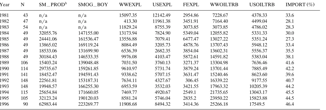
The 1997 Annual Energy Review prepared by the Energy Information Adminis-tration provides data on oil imports as a fraction of total US oil consumption ŽIMPORT . Descriptive statistics on data obtained from both datasets appear in. Table 1.
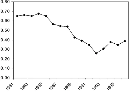
As noted above, exploration activity has shifted abroad while imports of oil have increased as a fraction of total US oil consumption. Figs. 1᎐3 provide some insight into these shifts. Fig. 1 shows that IMPORT has increased from a low of about 0.27 Žor, 27% in the early 1980’s to a recent high of 0.46. Fig. 2 shows that exploration.
Ž
dollars invested in US exploration USEXPL, defined as the sum of USDRL and
. Ž
USACQ by the sample firms as a fraction of worldwide exploration WWEXPL, .
defined as the sum of WWDRL and WWACQ has decreased from around 0.65 Žor, 65% in the early 1980’s to about 0.40 in recent years. Fig. 3 shows that US oil.
Ž . Ž .
reserves USOILTRB as a fraction of worldwide oil reserves WWOILTRB Ž owned by the sample companies decreased during the period from about 0.55 or,
.
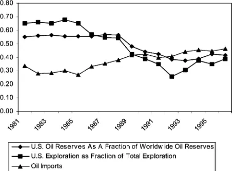
55% to about 0.42. Finally, Fig. 4, an overlay of Figs. 1᎐3, reveals the clear intertemporal association between reduced US exploration investment, reduced holdings of US reserves, and increased reliance on imported oil.
I evaluate the statistical significance of these trends by estimating the following regression model in which the slope coefficient on TIME forms a test of the null
Ž
hypothesis that the dependent variable,Y, either IMPORT, USEXPLrWWEXPL, .
()
Year N SM PRODᎏ SMOG BOYᎏ WWEXPL USEXPL FEXPL WWOILTRB USOILTRB IMPORT %
1981 43 nra nra 15097.35 12142.49 2954.86 7228.67 4378.33 33.6
1982 47 nra nra 413.30 11961.38 3451.91 7164.40 4499.04 28.1
1983 54 nra nra 11829.24 8755.39 3073.85 3073.85 4786.02 28.3
1984 49 32055.76 147155.00 13173.94 7824.90 5349.04 12055.82 5331.33 30.0
1985 49 24441.06 161536.47 13556.88 7079.41 6477.47 13027.22 5351.24 27.3
1986 49 13865.02 169119.24 8084.49 3205.73 4878.76 13707.43 5948.12 33.4
1987 49 18533.06 131699.90 6536.39 2682.35 3854.04 13602.31 5556.37 35.5
1988 49 30184.43 146533.35 9976.08 4103.47 5872.61 14591.82 5383.04 38.1
1989 106 15403.24 139048.48 7031.50 3760.13 3271.37 13304.98 7636.46 41.6
1990 114 29735.67 159261.85 9610.97 5731.74 3879.24 13701.44 7885.49 42.2
1991 141 18452.47 194591.43 9338.62 5707.15 3631.47 15240.46 8623.60 39.6
1992 148 22561.81 153187.31 7634.11 4327.67 306.45 16339.22 9177.55 40.7
1993 148 19948.57 166255.30 6953.59 3532.03 3421.55 17963.32 10205.39 44.2
1994 115 25654.84 171660.05 7469.77 4920.67 2549.1 21735.65 13043.17 45.5
1995 105 32123.24 190120.03 8581.24 5746.04 2835.2 23950.22 15823.88 44.5
1996 90 62983.44 223269.77 11908.68 8494.32 3414.36 25266.18 17549.5 46.4
a
Note: all amounts are in thousands. b
SM PROD is the present value of future net cash flows expected to be received from oil and gas reserves discovered during the current financialᎏ
reporting period. Expected net cash flows are discounted at a 10% discount rate; SMOG BOY is the present value of future net cash flows expected to beᎏ
received from oil and gas reserves owned at the beginning of the financial reporting period. Expected net cash flows are discounted at a 10% discount rate; WWDRL is the amount invested during the financial reporting period to drill for oil and gas worldwide; USDRL is the amount invested during the financial reporting period to drill for oil and gas in the United States; WWACQ is the amount invested during the financial reporting period to acquire exploration rights to property worldwide; USACQ is the amount invested during the financial reporting period to acquire exploration rights to property in the United
Ž .
States; WWOILTRB is the number of barrels of oil owned by the firm worldwide at the beginning of the financial reporting period; USOILTRB is the
Ž .
Fig. 1. Oil imports as a fraction of total oil consumed in US.
Ž .
Yts␣0q␣1TIMEqt 1
TIME is a time trend variable assigned a value of 1 if the observation occurred in 1981, a value of 2 if the observation occurred in 1982, and so on.
The adjusted R2 from the regression in which the dependent variable is
Ž . Ž .
IMPORT is 0.83, and the slope coefficient t-statistic on time is 0.0128 8.71 and statistically different from zero at the 0.001 level of significance. The adjusted R2
from the regression in which the dependent variable is USDRLrWWDRL is 0.80,
Ž . Ž .
and the slope coefficient t-statistic on time isy0.02767 y7.87 and statistically different from zero at the 0.001 level of significance. Finally, the adjusted R2 from
the regression in which the dependent variable is USOILTRBrWWOILTRB is
Ž . Ž .
0.74, and the slope coefficient t-statistic on time is y0.01402 y6.74 and
( )
J.P. BoonerEnergy Economics 23 2001 211᎐226 217
Fig. 3. US oil reserves as a fraction of worldwide oil reserves.
statistically different from zero at the 0.001 level of significance. These simple time-trend regressions suggest that US reliance on imported oil has increased
Ž .
across time while 1 the dollars invested to develop oil and gas reserves in the US; Ž .
and 2 US oil reserves as a fraction of worldwide oil reserves have both decreased across time. Each of these trends is consistent with the idea that reduced US exploration investment may have contributed to increased reliance on imported oil. The question this paper seeks to answer is whether lower returns on US ex-ploration investment, relative to returns earned on non-US exex-ploration investment,
might explain the migration of exploration capital abroad. The following section describes the empirical model used to help answer this question.
3. Empirical model used to estimate the present value of exploration investment
3.1. Methodology
Since exploration expenditures are made to yield future cash flows, the value of the exploration investment is the present value of the future cash flows that exploration yields. This value can be estimated by associating exploration expendi-tures of a given period with the present value of the future cash flows of reserves discovered in a subsequent year. In particular, I specify the present value of oil and gas reserves discovered in year t as a function of current and lagged exploration expenditures:
L L
Ž . SM PRODᎏ i ts␣0q
Ý
␣1,kUSEXPLi tykqÝ
␣2,kFEXPLi tykqi t 2ks0 ks0
USEXPL is defined as the sum of USDRL and USACQ, while FEXPL is defined as WWDRLqWWACQ-USEXPL. The slope coefficient ␣1,k measures the dollar value of reserves discovered in year t from $1 invested in US exploration during year tyk, and ␣2,k measures the dollar value of reserves discovered in year t from $1 invested in non-US exploration during year tyk. The length of the lag, L, indicates the period of time necessary to complete an exploration project. The present value of the return earned from the exploration investment is calculated by discounting the slope coefficients at a rate of interest, r, that reflects the risk of the firm’s exploration activity. So, the present value of $1 invested in US exploration is calculated as
and the present value of $1 invested in non-US exploration is calculated as
L ␣
To help mitigate the multicollinearity problem inherent in estimating the model
Ž . Ž .
as specified in 2 , I estimate model 2 as a degree 2 polynomial distributed lag. This approach, based on the assumption that the distribution of lag coefficients can be approximated as: ␣ s q kq k2; and ␣ s␦ q␦ kq␦ k2,
re-1,k 0 1 2 2,k 0 1 2
U
Ž . Ž
duces the number of parameters that must be estimated from 2 Lq1 to six 0, .
( )
J.P. BoonerEnergy Economics 23 2001 211᎐226 219
␣2,k. Similarly, the covariance matrix of ␣1,k, ␣2,k is obtained from the covariance
Ž . Ž .
matrix of 0, 1, 2, ␦0, ␦1, ␦2. See Almon 1965 and Greene 1997 for further details.
Ž .
Since the variables in 2 are undeflated, I control for size-related coefficient bias by including SMOG BOY as a regressor and base statistical inferences onᎏ
Ž .
White 1980 heteroskedasticity-consistent covariance matrix. I also control for firm-specific and time-specific fixed-effects by including firm and time dummies. Thus, the empirical model that I estimate is:
SM PRODᎏ i ts0iq1tq2SMOG BOYᎏ i t
Model 5 is estimated by pooling firm-specific cross-sectional observations taken from the Arthur Andersen Reserve Disclosures Database across the period 1981᎐1996. The length of the lag, L, is based on the lag yielding the best ‘fit’ as assessed by the model R2 and the standard errors of the coefficients. The slope coefficients  and ␦ are retained and used to calculate the lag coefficients ␣1,k,
␣2,k, which are then discounted at a 10% rate of interest to yield point estimates of PVUSEXPL and PVFEXPL. The discount rate of 10% is chosen to retain consistency with the calculation of SM PROD.ᎏ
Ž . Ž .
Two additional aspects about model 5 warrant elaboration. First, model 5 constrains dollars invested outside the US to generate identical returns. For example, $1 invested in Country A is assumed to generate the same return as $1 invested in Country B. This simplifying assumption was necessary because firms generally do not report to shareholders country-specific information on exploration investment and reserve disclosures. To the extent this assumption is materially
Ž .
inaccurate, model 5 is misspecified. Second, exploration technology undoubtedly has changed across the past 15 years, and this change in technology may well have
Ž .
impacted returns on exploration investment. Model 5 attempts to control for the effects of any intertemporal change in technology on returns to exploration investment by including year dummy variables.
3.2. Results
Ž .
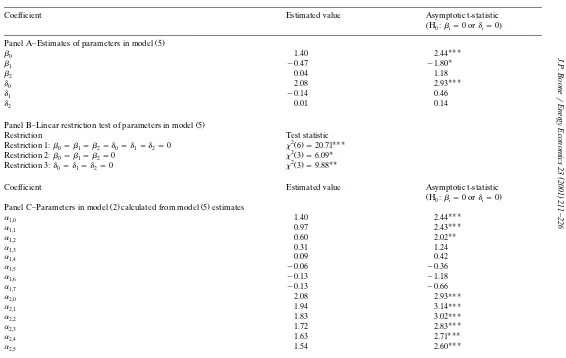
Empirical estimates of model 5 and related tests of coefficients are presented in Panels A and B of Table 2, while the lag coefficients calculated from the estimates in Panel A and related tests of coefficients are summarized in Panels C
Ž .
and D. Turning first to Panels A and B, we see that model 5 exhibits generally good fit, with the null hypothesis that 0s1s2s␦0s␦1s␦2s0 strongly
Ž 2 .
re-()
Panel A᎐Estimates of parameters in model 5
UUU
Panel B᎐Linear restriction test of parameters in model 5
Restriction Test statistic
Panel C᎐Parameters in model 2 calculated from model 5 estimates
()
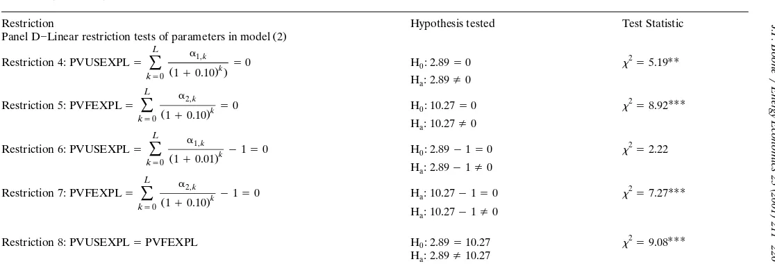
Panel D᎐Linear restriction tests of parameters in model 2
L ␣
Restriction 8: PVUSEXPLsPVFEXPL H : 2.890 s10.27 s9.08
H : 2.89a /10.27
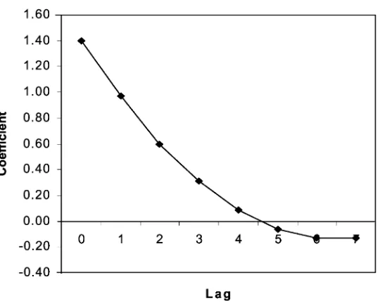
aU UU UUU Ž .
Fig. 5. Lag coefficient for US exploration investment.
Ž 2 .
jected s6.09, Ps0.10 , and the null hypothesis that ␦0s␦1s␦2s0
re-Ž 2 .
jected s9.88, Ps0.05 .
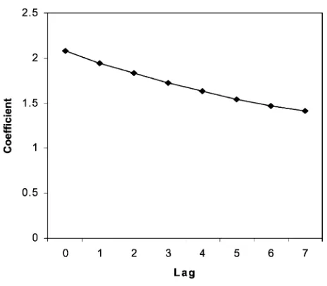
Panel C shows that the lag coefficients ␣1,k are statistically significant for lags 0 through 2, while the lag coefficients a2,k are statistically significant for lags 0 through 7. Figs. 5 and 6 graphically depict the estimated slope coefficients ␣1,k and
␣2,k, revealing that both ␣1,k and ␣2,k decline monotonically through lag 7. The slope coefficients ␣1,k when discounted at 10% yields an estimated value of PVUSEXPl of $2.89, which is statistically distinguishable from zero at the 0.05
Ž .
level of significance Panel D, restriction 4 . Similarly, the slope coefficients ␣2,k
when discounted at 10% yield an estimated value of PVFEXPL of $10.27 which is Ž
statistically distinguishable from zero at the 0.01 level of significance Panel D, .
Restriction 5 .
Restriction tests 6 and 7 evaluate whether exploration is a positive net present
Ž .
value project that is, whether PVUSEXPLy1)0 and PVFEXPLy1)0 . Restriction 6 is unable to reject the null hypothesis that PVUSEXPLy1s0 while, in contrast, restriction 7 is able to reject the null hypothesis that PVFEXPL y1s0. Thus, restriction 7 indicates that investment in non-US exploration is a positive net present value project, but restriction 6 is unable to reject the null hypothesis that US exploration investment is not a positive net present value project.
ex-( )
J.P. BoonerEnergy Economics 23 2001 211᎐226 223
Fig. 6. Lag coefficient for non-US exploration investment.
ploration yields the same present value return as a dollar invested in non-US exploration, is rejected, thus indicating that non-US exploration investment yields a greater present value return than investment in US exploration.
Overall, the results reported in Table 2 provide evidence suggesting that non-US exploration is a higher positive net present value project than is US exploration, implying the possibility that exploration capital has migrated abroad in search of higher returns on investment. An alternative explanation, however, is that the higher net present value of non-US exploration investment represents a risk premium to compensate firms for accepting the additional risk associated with non-US exploration, and thus, risk-adjusted returns to non-US exploration are the
Ž .
same as or perhaps even less than US exploration. To probe the plausibility of this alternative explanation, I compare the mean lag for US exploration investment to the mean lag for non-US exploration. The mean lag is an approximate measure of the number of years that it takes for one-half of the benefits from the investment to be realized. Under the assumption that investments that pay off
Ž sooner rather than later are in some sense less risky, the exploration province US
.
or non-US with the greater mean lag will be interpreted as ‘riskier.’ The mean lag of the jth exploration province is defined as
L
Ž .
mean lagjs
Ý
kwjk 6where
␣jk
Ž .
wjks L 7
␣
Ý
jkks0
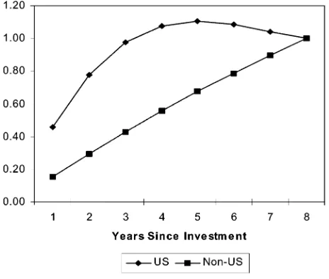
The mean lag for US exploration investment is 0.48 years, while the mean lag for non-US exploration investment is 3.2 years. Fig. 7, which plots the cumulative proportion of benefits received from exploration investment as a function of time, provides an intuitive interpretation of these mean lags. As Fig. 7 shows, approxi-mately 50% of the reserves yielded by a $1 investment in US exploration have been discovered within approximately 1 year after the investment, while it takes between 3 and 4 years to discover 50% of the reserves yielded by a $1 investment in non-US exploration. Thus, the mean lag as a measure of exploration risk indicates that non-US exploration investment is riskier than US exploration investment. In turn, this suggests that at least some of the excess net present value earned on non-US exploration investment represents a premium to compensate for the heightened risk associated with non-US exploration. Unfortunately, the research design does not permit one unambiguously to infer whether all of the excess net present value
Ž
earned on non-US investment represents risk premium implying that the risk-adjusted returns to US exploration investment and non-US exploration investment
.
are the same , or whether only a portion of the excess net present value earned on Ž
non-US investment represents risk premium implying that the risk-adjusted re-turns to non-US exploration investment exceed those earned on US exploration
. investment .
( )
J.P. BoonerEnergy Economics 23 2001 211᎐226 225
4. Concluding comments
This paper documents the relative magnitude of returns to investment in US vs. non-US exploration provinces. The empirical evidence presented in the paper indicates that the net present value of $1 invested in non-US exploration is larger in a statistically significant sense than the net present value of $1 invested in US exploration. In particular, results indicate that the return on non-US exploration investment is approximately 3.5 times as large as the return earned on US exploration investment. Furthermore, statistical tests revealed that investment in non-US exploration is a positive net present value project while tests failed to indicate that investment in US exploration is a positive net present value project. These findings are important because they may help energy policymakers to intelligently devise what action, if any, is warranted in response to the growing reliance of the US on oil imported from abroad. For example, the order of magnitude of the differences between US and non-US return on exploration investment documented in this paper suggests that it is highly unlikely that tax policy could be effectively used to stimulate domestic US exploration by providing tax preferences targeted to US exploration.
The results documented in this study must be interpreted in light of two important limitations. First, the net present values from exploration investment that were calculated in this study are based exclusively on pri¨ate costs incurred by the individual firm and exclude the social costs to US citizens of maintaining a military presence in oil-rich provinces abroad to defend US access to imported oil. While managers of US oil firms presumably calculate net present values in the
Ž .
same fashion considering only private costs and ignoring social costs , the inability to include social costs in the analysis implies that the estimates of net present value from non-US exploration are biased upward. Thus, if the results documented in this study are accepted at face value and one concludes that US exploration capital has migrated abroad in search of higher returns on pri¨ateinvestment, one cannot necessarily conclude that this flow of capital is economically efficient nor socially desirable since capital is being allocated based on an incomplete measure of the total cost of non-US exploration investment.
Second, evidence suggests that non-US exploration investment is riskier than US
Ž .
exploration investment, and thus, some portion or all of the excess of net present value on non-US investment over the net present value earned on US investment may be attributable to risk premium. Thus, while, the empirical results documented in this paper suggest that the risk-neutral return on non-US investment is 3.5 times as large as that earned on US investment, risk-adjusted returns earned on non-US investment may exceed the risk-adjusted returns earned on US exploration invest-ment by a much smaller order of magnitude.
References
Ž .
Amoco Corporation, 1990 . Report to U.S. Department of Energy. Cited in Platt’s Oilgram News.
Ž .
68 93 , 6.
Bertagne, R., 1988. International exploration by independents. Oil Gas J. 22, 62.
Eiteman, D., Stonehill, A., 1986. Multinational Business Finance, 4th Edition. Addison-Wesley Publish-ing Company, Massachusetts.
Ž .
Fatemi, A., 1984. Shareholder benefits from corporate international diversification. J. Fin. 39 5 , 1325᎐1345.
Ž .
Financial Accounting Standards Board. 1977 . Statement of financial accounting standards no. 19. Stamford, CT: Financial Accounting Standards Board.
Ž .
Financial Accounting Standards Board. 1982 . Statement of financial accounting standards no. 69. Stamford, CT: Financial Accounting Standards Board.
Greene, W., 1997. Econometric Analysis. Prentice-Hall, Upper Saddle River, New Jersey.
Griffian, J., Karolyi, G., 1998. Another look at the role of the industrial structure of markets for
Ž .
international diversification strategies. J. Financ. Econ. 50 3 , 351᎐373.
Ž .
Oil and Gas Journal, 1998. Exxon-Mobil Total-Petrofina mergers slated. Oil Gas J. 96 49 , 37᎐42.
Ž .
US Department of Energy, Energy Information Administration, 1991 . Average effective corporate
Ž .
income tax rates for petroleum operations 1977᎐1999. DOErEIA-0550 . Washington, D.C.: U.S. Department of Energy, Energy Information Administration.
Wasteneys, R., 1997. Strategic choices crucial to foreign upstream ventures. Oil Gas J. 10, 49.
Ž .
Weston J, B. Johnson, J. Siu. 2000 . Mergers and restructuring in the world oil industry’. J. Energy Fin.
Ž .
Dev. forthcoming .