Dengfeng Chaia, Alena Schmidtb, Christian Heipkeb
aInstitute of Spatial Information Technique, Zhejiang University, China [email protected]
b
Institute of Photogrammetry and GeoInformation, Leibniz Universit¨at Hannover, Germany [email protected], [email protected]
ICWG III/VII
KEY WORDS:Linear Feature, Feature Detection, Spatial Point Processes, Global Optimization, Simulated Annealing, Markov Chain Monte Carlo
ABSTRACT:
This paper proposes a novel approach for linear feature detection. The contribution is twofold: a novel model for spatial point processes and a new method for linear feature detection. It describes a linear feature as a string of points, represents all features in an image as a configuration of a spatial point process, and formulates feature detection as finding the optimal configuration of a spatial point process. Further, a prior term is proposed to favor straight linear configurations, and a data term is constructed to superpose the points on linear features. The proposed approach extracts straight linear features in a global framework. The paper reports ongoing work. As demonstrated in preliminary experiments, globally optimal linear features can be detected.
1. INTRODUCTION
Image features play a fundamental role in many tasks of image analysis. For example, both surface reconstruction and object extraction usually rely on some distinguishable features. Fea-ture detection has been investigated widely in the communities of photogrammetry and remote sensing, computer vision and pat-tern recognition. However, few works were dedicated to model-ing feature shape in a global framework. This paper address this issue in the context of detecting linear features. Linear features offer salient cues for region boundaries and object contours.
1.1 Related Work
Image features refer to image primitives such as points, lines, curves and regions. Corner detectors and interest point detectors have been developed to detect point features (F¨orstner and G¨ulch, 1987, Harris and Stephens, 1988, Tomasi and Kanade, 1991, Shi and Tomasi, 1994, Smith and Brady, 1997, Lowe, 2004, Ros-ten and Drummond, 2006, Bay et al., 2008, Rublee et al., 2011). Region detectors have been proposed to detect region features (Kadir et al., 2004, Tuytelaars and Van Gool, 2004, Leutenegger et al., 2011, Alahi et al., 2012). Both straight lines and curves are linear features. Their detection is formulated as edge detection, line detection, boundary detection or contour detection.
Edge detection aims at detecting edges, which refer to abrupt changes of brightness. Basically, sharp changes are computed by differential operations, which is achieved by differentiation based filters such as Sobel, Prewitt, Roberts, Laplacian of Gaus-sian, etc. These filters are simple and sensitive to noise. This disadvantage is significantly overcome by the Canny edge de-tector (Canny, 1986). Its success depends on the definition of three comprehensive criteria, namely good detection, good local-ization and single-pixel response, for the computation of edges. Edge detection is formulated as an optimization with respect to these criteria. Benefiting from its solid mathematical foundation, this detector has proven to be reliable and has gained popular-ity since it was first published. Besides, there are some extended and adapted versions (Deriche, 1987, McIlhagga, 2011, Xu et al.,
2014). However, feature shape is not modeled in the computa-tional framework.
Lines are pairs of anti-parallel edges. Depending on the width of the linear feature to be detected and the contrast with respect to the neighborhood, line detection can be advantageous to edge detection. The most prominent example of line detection is the Steger operator (Steger, 1998).
Boundary detection refers to detecting boundaries between differ-ent regions. Boundaries are indicated by edges, excluding those inside a region. However, there are typically a lot of edges inside a textured region. This issue is addressed by the Pb (probability-of-boundary) edge detection algorithm (Martin et al., 2004). For each pixel it fuses brightness gradient, texture gradient and color gradient to calculate the probability of being a boundary pixel. Further, MS-Pb (Multiple Scale Pb) integrates Pb in multiple scales (Ren, 2008), and gPb (global Pb) introduces global infor-mation into the MS-Pb (Arbelaez et al., 2011). The gPb detector can detect boundaries between texture regions. However, none of them models boundary shape.
Contour detection is dedicated to extracting outlines of objects of interest. Some approaches group edges, lines or boundary frag-ments into contours (Zhu et al., 2007, Arbelaez et al., 2011, Ming et al., 2013, Payet and Todorovic, 2013). The other approaches fit active contour models to images (Kass et al., 1988, Mishra et al., 2011, Dubrovina et al., 2015). Although shape is modeled and utilized by these approaches, modeling is performed not in a global framework.
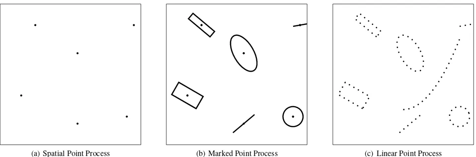
(a) Spatial Point Process (b) Marked Point Process (c) Linear Point Process
Figure 1: Overview of three kinds of spatial point processes.
marks are too specific to represent general linear shapes. Al-though a combination of above marks integrates their capacities (Lafarge et al., 2010), they are not general enough to represent freeform linear features. Alternatively, stochastic models can be employed to segment an image into regions, whose boundaries are freeform linear features (Tu and Zhu, 2002). However, re-gions instead of boundaries are modeled explicitly.
1.2 Motivation and Contribution
Most feature detectors are not developed in a global framework. Also, they do not deal with feature shape and uncertainty. While marked point processes do provide a global model for feature shape and uncertainty, in existing approaches linear features are represented by geometric marks. Apart from losing generality, the space of solutions is expanded significantly since additional parameters are involved in decribing the geometric marks. These additional parameters impair both detection quality and efficiency.
With reference to Fig. 1 a point is an atomic element in math-ematics, and a string of points forms a (possibly straight) curve. In turn, a set of connected curves encloses a region. Motivated by this common sense observation, in this paper a linear feature is represented by a string of points. Further, the paper proposes a spatial point process, in which points are inclined to form curves as shown in Fig. 1(c). The paper makes several contributions:
• Spatial point process:Based on the proposed model for a spatial point process, points can form linear shapes. This characteristic assures its potential in modeling and analyz-ing linear shapes.
• Feature representation: The proposed model is general enough to represent freeform linear features. Edges, lines, boundaries and contours can all be represented in this model.
• Global feature detection: Linear feature detection is for-mulated as a global optimization problem. The globally op-timal solution can be reached very efficiently since no extra parameters are involved in the computation.
The rest of the paper is organized as follows. First, some back-ground information on spatial point processes is introduced in Sec. 2 Second, the novel approach for linear feature extraction is proposed in Sec. 3 Then, experimental results are presented in Sec. 4 Finally, conclusions are drawn in Sec. 5
2. FEATURE EXTRACTION BASED ON MARKED POINT PROCESSES
2.1 Spatial Point Processes
A spatial point process is a useful model for a random pattern of points as depicted in Fig. 1(a). For ak-dimensional spaceRk, letF ⊂Rkbe a compact set, letω={ω1, . . . , ωn}be a
config-uration havingnunordered pointsωi ∈ F, letΩnbe the set of
configurations that consist ofnpoints. A point process onF is a mappingΨfrom a probability space to the set of configurations Ω =S∞
n=1Ωn, such that, for all bounded Borel setsS⊂F, the
number of pointsNΨ(S)falling inSis a finite random variable.
A Poisson process in the plane with uniform intensity measure
ν(.)is a point process inF ∈R2, such that, for every bounded closed set S ∈ F, the number of points falling in this region follows a Poisson distribution with meanν(S), and the number of points are independent for disjoint regions.
Complex point processes are specified by a probability density
h(.)defined onΩand a reference measureµ(.)under the condi-tion that the normalizacondi-tion constant ofh(.)is finite:
Z
ω∈Ω
h(ω)dµ(ω)<∞. (1)
The measureµ(.)having the densityh(.)is usually defined via the intensity measureν(.) of a homogeneous Poisson process. For a more detailed definition of point processes the reader is referred to (Møller and Waagepetersen, 2004).
2.2 Feature Extraction Based on Marked Point Processes To extract features from images, a data term measuring the con-sistency between the points and the image is introduced into the densityh(.), and a prior term reflecting the spatial interactions among the points is also introduced into the density. This density can be expressed as a product of a data termhd(.)and a prior
termhp(.):
h(.) =hp(.)hd(.). (2)
Feature extraction is achieved by searching for the configuration
ω⋆maximizing the probability density as
ω⋆= arg max
ω∈Ω
geometric marks are very specific, they cannot represent general shapes. Furthermore, the configuration spaceΩis expanded dra-matically by the extra parameters for the marks. Both, detection quality and efficiency are impaired within this complex space.
3. LINEAR FEATURE EXTRACTION BASED ON SPATIAL POINT PROCESSES
3.1 Linear Feature Representation
This paper represents a linear feature by a string of points instead of a geometric mark. As shown in Fig. 1(c), a line segment is represented by a set of points sampled on the segment. Any other linear features such as freeform curves are also represented by their sample points.
The suggested model contains a data term measuring the consis-tency between the points and the image data. Further, this paper proposes a prior model for spatial point processes such that linear configurations become more probable than non-linear configura-tions and straight ones are prefered to curved ones.
3.2 A Prior Model for Linear Configurations
A prior probability of a configurationωis measured by three dif-ferent criteria: the sparsity of its points, the neighborhood of its points and the curvature of the linear configuration. The density
hpis a product of three densities:
hp(ω)∝hs(ω)hnb(ω)hc(ω), (4)
wherehs(ω),hnb(ω)andhc(ω)are three densities based on the
criteria of sparsity, neighborhood and curvature, respectively.
Figure 2: Sparsity is assured by penalizing closely neighboring points indicated by the overlapping disks.
Sparsity: Configurations of sparse points are assured by penal-izing small distances between neighboring points. Let a disk of radiusr1be the influence area of each point as illustrated in Fig. 2. When two points are closer than2r1, their disks overlap. To avoid overlapping, the distance between any two points must be larger than2r1.
The density for sparsity is defined as
hs(ω)∝αs(ω,r1), (5)
whereαis a parameter of this model,s(ω, r1)is calculated as
follows:
ωi,ωj∈ω
whered(ωi, ωj)is the distance betweenωiandωj.
The above model penalizes small distances between neighboring points. For0< α <1, it is a soft constraint, points are allowed to be closer than2r1, but they are less probable.
ωi
ωj
ωk
Figure 3: Each point on a line excluding the first and last point has two neighbors within a disk, i.e., a preceding point and a succeeding point.
Neighborhood: As one tracks points along a line, each point has a preceding point and a succeeding point, excluding the first point and the last point. As depicted in Fig. 3, pointωjhas a preceding
pointωiand a succeeding pointωk. This is a basic characteristic
of linear features; it is introduced into the neighborhood density as follows
hnb(ω) =βnb(ω,r2), (7)
whereβis a parameter of this model, andnb(ω, r2)is calculated
as
nb(ω, r2) = X
ωj∈ω
|deg(ωj, r2)−2|, (8)
wheredeg(ωj, r2)is the degree ofωj, i.e. the number of points
within a disk of radiusr2around ωj. Note that typicallyr2 is
assumed to be larger thanr1.
deg(ωj, r2) =
X
ωi∈ω,ωi6=ωj
1[d(ωi, ωj)≤r2], (9)
whered(ωi, ωj)is the distance betweenωiandωj.
For0< β <1, points with two neighbors within a disk of radius
r2are preferred and the other points are penalized.
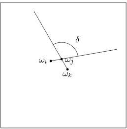
Curvature: The local curvature at a point of a linear feature is described by the angleδdefined by its preceding and succeeding point as illustrated in Fig. 4. Note that the curvature term is only applied for points with exactly two neighbors, as otherwise its computation in the described way is either not possible (one neighbor) or ambiguous (three or more neighbors).
δ
ωi ωj
ωk
Figure 4: The angle defined by three successive points.
turn, small curvature is indicated by an angle close toπ. This angle is introduced into the curvature density as follows
hc(ω) =γc(ω), (10)
For0< γ <1, points with large curvature are penalized.
3.3 Data Consistency of Linear Features
Assuming the data for the points to be independent, the data den-sity can be written as a product of local terms
hd(ω)∝
Y
i=1,2,...n
hd(ωi), (13)
where the local termhd(ωi)for a pointωimeasures its
consis-tency with a linear feature, i.e. the likelihood of being either a corner or an edge. The local term is computed by
hd(ωi) = exp(λ1+λ2), (14)
whereλ1andλ1are two eigenvalues of the Harris matrix, which is calculated as the covariance matrixMof the derivatives of the imageIwith respect to the pixel neighborhood
M = measuring the flatness at the point. Large values indicate either a corner or an edge. Therefore, this data term can be used to find points at object boundaries.
3.4 Linear Feature Extraction
Linear feature extraction is formulated as finding the optimal con-figuration of a spatial point process. The optimal concon-figuration
ω⋆maximizes the probability density
ω⋆= arg max
ω∈Ω
hs(ω)hnb(ω)hc(ω)hd(ω). (16)
This is not a conventional optimization problem since the con-figuration space has variable dimensions and the probability den-sity is multi-modal. Simulated annealing is employed to succes-sively simulate a series of probability distributions which con-verges to a distribution concentrated on the optimal configuration (Kirkpatrick et al., 1983). The Reversible Jump Markov Chain Monte Carlo (RJMCMC) sampler is embedded into the optimiza-tion procedure to take into account the variable dimension of the configuration space and to simulate the expected probability dis-tribution (Green, 1995).
3.4.1 Searching the Optimal Configuration: Consider a spa-tial point process, in which each configurationωhas the proba-bility density
hT(ω) = [h(ω)]1/T = [hs(ω)hnb(ω)hc(ω)hd(ω)]1/T, (17)
whereT >0is a temperature parameter. WhenT → ∞,hT(ω)
defines a uniform distribution onΩ; forT = 1,hT(ω) =h(ω);
and asT → 0, hT(ω) concentrates on the optimal
configura-tionω⋆. When the temperature starts from a large value and de-creases according to a logarithmic function, it is guaranteed that the globally optimal configuration is found as the temperature ap-proaches zero. In practice, a faster geometric decrease gives an approximate solution, in general close to the optimum (Baddeley and Lieshout, 1993).
The RJMCMC sampler is adopted to simulate a discrete Markov Chain(Xt)t∈N, which converges tohT(ω). At each transition,
one point of the current configurationωis perturbed to generate a new configurationω′
according to a kernelQ(ω→.). The con-figurationω′is then accepted as the new state of the chain with a probabilitymin(1, R), in which the Green ratio is calculated as
R=Q(ω
The kernelQcan be a mixture of some sub-kernelsQm
Q(ω→.) =X
m
pmQm(ω→.), (19)
wherepmis the probability of choosing the sub-kernelQm.The
kernel mixture must allow any configuration inΩto be reached from any other configuration in a finite number of perturbations (irreducibility condition of the Markov chain), and each sub-kernel has to be reversible, i.e. able to propose the inverse perturbation.
3.4.2 Transition Kernels: The birth and death kernelQBD
and the translation kernelQTare developed in the sampler. These
from the current configurationω, respectively. Adding and re-moving a point corresponds to jumps into a higher dimensional and a lower dimensional subspace, respectively. The green ratio for a birth kernel is given by
R= pdλF
where λF is the Poisson parameter representing the expected
number of points in the domainF (the whole image), n(ω′) is the number of points in the proposed configurationω′, ωi′ is
the inserted point, andpd(resp. pb) is the probability of
choos-ing a death (resp. a birth) kernel. In our experiments we set
pd =pb = 0.5. In case of a death, the proposition kernel ratio
corresponds to the inverse of the birth’s ratio.
Translation kernel:The translation kernel moves a pointωito a
new pointωi′. The green ratio for a translation kernel is given by
R=
In our experiments, a point is moved in a square centered around its old position and the length of each side is set to ber1.
3.4.3 Sampling Driven by Gradients: The above scheme sam-ples the configuration space uniformly. It spends a lot of time checking impossible configurations. The points are usually ex-pected to lie on edges with large gradients. Motivated by the Data Driven Markov Chain Monte Carlo (DDMCMC) approach (Tu and Zhu, 2002), a scheme utilizing gradient information is developed to improve the sampling.
First, the point must be sampled at the pixel locations, i.e. the sample points stem from the set of pixels:
ωi∈P, (22)
wherePis the set of pixels.
Then, each pixel has a weight proportional to its gradient magni-tude
w(p)∝qI2
x+Iy2, (23)
whereIx= ∂I∂xandIy= ∂I∂yare the two derivatives. The weights
of all pixels are normalized such that its sum equals one.
Finally, uniform birth and death is replaced with gradient driven birth and death. In uniform birth and death, each pixel has the same chance of being selected as a new point, while in gradient driven birth and death the pixels having larger gradient have more chance of being selected as a new point. The chance is propor-tional to its gradient.
The described method was implemented and some preliminary tests were conducted to obtain a first insight into the behavior of the suggested approach. The experiments consist of model simu-lation and feature detection, the results are reported in the follow-ing. The parameters selected for the experiments are presented in Tab. 1.
λ α β γ r1(pixels) r2(pixels)
200 0.9 0.9 0.9 5 10
Table 1: Parameters for experiments
Fig. 5 presents two simulations based on two models. An optimal configuration based on the homogenous Poisson point process is presented in the left figure. The points are totally random and no linear features appear. In contrast, the right figure presents an optimal configuration based on the proposed model. The points are inclined to form lines and curves as expected.
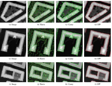
Fig. 6 presents the results of feature detection. The left column presents the original images. The two middle columns depict features detected by the Harris detector (Harris and Stephens, 1988) and the Canny detector (Canny, 1986). The right col-umn depicts features detected by the proposed approach. The detected features are represented by the shown points. The de-tected points representing the linear features are well placed on the region boundaries and they clearly illustrate the outline of the objects. Moreover, they are general enough to represent any freeform features and objects.
The data term is calculated once for each pixel and is stored as an image for use in the sampling procedure. In this way calculation efforts are minimized and a better efficiency is achieved.
5. CONCLUSION
This paper proposes a novel approach for linear feature detection. Feature detection is formulated as finding an optimal configura-tion of a spatial point process. Based on this formulaconfigura-tion, a prior model is proposed to favor straight linear configurations, and a data model is constructed to draw the points towards linear fea-tures. The proposed approach detects linear features in a globally optimal framework. As demonstrated by the experiments, fea-tures can in principle be detected and they sit on the boundaries with good accuracy.
One limitation of the approach is that linear features are not de-tected explicitly. The model can only serve as an intermedi-ate representation between edges and contours, which are low-level and high-low-level features, respectively. Converting the de-tected points into contours is worthy to investigate in the future. Further, the model does not include any topological constraints. Therefore, a network containing junctions cannot be properly ex-tracted. Representing junctions without marks is also an issue which needs further attention. Finally, the data term can be im-proved by introducing a more sophisticate response, e.g. by in-troducing the concep of probability-of-boundary (Martin et al., 2004).
ACKNOWLEDGEMENTS
(a) Poisson (b) Linear
Figure 5: Two simulation results: on the left an optimal configuration of a homogenous Poisson point process is shown, in which points are distributed randomly. To the right a configuration with density defined by the proposed model is illustrated, in which points are distributed along linear curves.
(a) Image (b) Harris (c) Canny (d) SPP
(e) Image (f) Harris (g) Canny (h) SPP
(i) Image (j) Harris (k) Canny (l) SPP
Alahi, A., Ortiz, R. and Vandergheynst, P., 2012. Freak: Fast retina keypoint. In: 2012 IEEE Conference on Computer Vision and Pattern Recognition (CVPR), pp. 510–517.
Arbelaez, P., Maire, M., Fowlkes, C. and Malik, J., 2011. Con-tour detection and hierarchical image segmentation. IEEE Trans-actions on Pattern Analysis and Machine Intelligence 33(5), pp. 898–916.
Baddeley, A. J. and Lieshout, M. V., 1993. Stochastic geometry models in high-level vision. Journal of Applied Statistics 20(5-6), pp. 231–256.
Bay, H., Ess, A., Tuytelaars, T. and Van Gool, L., 2008. Speeded-up robust features (surf). Computer Vision and Image Under-standing 110(3), pp. 346 – 359. Similarity Matching in Computer Vision and Multimedia.
Canny, J., 1986. A computational approach to edge detection. IEEE Transactions on Pattern Analysis and Machine Intelligence (6), pp. 679–698.
Chai, D., F¨orstner, W. and Lafarge, F., 2013. Recovering line-networks in images by junction-point processes. In: IEEE Con-ference on Computer Vision and Pattern Recognition (CVPR), pp. 1894–1901.
Deriche, R., 1987. Canny’s criteria to derive a recursively imple-mented optimal edge detector. International Journal of Computer Vision 1, pp. 167–187.
Dubrovina, A., Rosman, G. and Kimmel, R., 2015. Multi-region active contours with a single level set function. IEEE Transac-tions on Pattern Analysis and Machine Intelligence 37, pp. 1585– 1601.
F¨orstner, W. and G¨ulch, E., 1987. A fast operator for detection and precise location of distinct points, corners and centres of cir-cular features. ISPRS Intercommission Conference on Fast Pro-cessing of Photogrammetric Data pp. 281–305.
Green, P. J., 1995. Reversible jump markov chain monte carlo computation and bayesian model determination. Biometrika 82(4), pp. 711–732.
Harris, C. and Stephens, M., 1988. A combined corner and edge detector. In: Alvey Vision Conference, Vol. 15, Citeseer, pp. 147– 151.
Kadir, T., Zisserman, A. and Brady, M., 2004. An affine invari-ant salient region detector. In: Computer Vision-ECCV 2004, Springer, pp. 228–241.
Kass, M., Witkin, A. and Terzopoulos, D., 1988. Snakes: Active contour models. International Journal of Computer Vision 1(4), pp. 321–331.
Kirkpatrick, S., Gelatt, C. D. and Vecchi, M. P., 1983. Optimiza-tion by simulated annealing. Science 220(4598), pp. 671–680.
Lacoste, C., Descombes, X. and Zerubia, J., 2005. Point pro-cess for unsupervised line network extraction in remote sensing. IEEE Transactions on Pattern Analysis and Machine Intelligence 27(10), pp. 1568–1579.
Lacoste, C., Descombes, X. and Zerubia, J., 2010. Unsupervised line network extraction in remote sensing using a polyline pro-cess. Pattern Recognition 43(4), pp. 1631–1641.
Lafarge, F., Gimelarb, G. and Descombes, X., 2010. Geomet-ric feature extraction by a multi-marked point process. IEEE Transactions on Pattern Analysis and Machine Intelligence 32(9), pp. 1597–1609.
tional Conference on Computer Vision (ICCV), pp. 2548–2555.
Lowe, D., 2004. Distinctive image features from scale-invariant keypoints. International Journal of Computer Vision 60(2), pp. 91–110.
Martin, D. R., Fowlkes, C. C. and Malik, J., 2004. Learning to detect natural image boundaries using local brightness, color, and texture cues. IEEE Transactions on Pattern Analysis and Machine Intelligence 26(5), pp. 530–549.
McIlhagga, W., 2011. The canny edge detector revisited. Inter-national Journal of Computer Vision 91(3), pp. 251–261.
Ming, Y., Li, H. and He, X., 2013. Winding number for region-boundary consistent salient contour extraction. In: 2013 IEEE Conference on Computer Vision and Pattern Recognition (CVPR), pp. 2818–2825.
Mishra, A. K., Fieguth, P. W. and Clausi, D. A., 2011. Decoupled active contour (dac) for boundary detection. IEEE Transactions on Pattern Analysis and Machine Intelligence 33(2), pp. 310– 324.
Møller, J. and Waagepetersen, R., 2004. Statistical inference and simulation for spatial point processes. Chapman & Hall/CRC.
Ortner, M., Descombes, X. and Zerubia, J., 2007. Building outline extraction from digital elevation models using marked point processes. International Journal of Computer Vision 72(2), pp. 107–132.
Ortner, M., Descombes, X. and Zerubia, J., 2008. A marked point process of rectangles and segments for automatic analysis of digital elevation models. IEEE Transaction on Pattern Analysis and Machine Intelligence 30(1), pp. 105–119.
Payet, N. and Todorovic, S., 2013. Sledge: sequential labeling of image edges for boundary detection. International Journal of Computer Vision 104(1), pp. 15–37.
Perrin, G., Descombes, X. and Zerubia, J., 2005. A marked point process model for tree crown extraction in plantations. In: Proc. of IEEE International Conference on Image Processing, pp. 1–4.
Ren, X., 2008. Multi-scale improves boundary detection in natu-ral images. In: Computer Vision–ECCV 2008, Springer, pp. 533– 545.
Rosten, E. and Drummond, T., 2006. Machine learning for high-speed corner detection. In: A. Leonardis, H. Bischof and A. Pinz (eds), Computer Vision - ECCV 2006, Lecture Notes in Com-puter Science, Vol. 3951, Springer, pp. 430–443.
Rublee, E., Rabaud, V., Konolige, K. and Bradski, G., 2011. Orb: an efficient alternative to sift or surf. In: 2011 IEEE International Conference on Computer Vision (ICCV), pp. 2564–2571.
Schmidt, A., Rottensteiner, F., Soergel, U. and Heipke, C., 2015. A graph based model for the detection of tidal channels using marked point processes. The International Archives of the Pho-togrammetry, Remote Sensing and Spatial Information Sciences XL-3/W3, pp. 115–121.
Shi, J. and Tomasi, C., 1994. Good features to track. In: IEEE Computer Society Conference on Computer Vision and Pattern Recognition, IEEE, pp. 593–600.
Smith, S. and Brady, J., 1997. Susan - a new approach to low level image processing. International Journal of Computer Vision 23(1), pp. 45–78.
Stoica, R., Descombes, X. and Zerubia, J., 2004. A gibbs point process for road extraction from remotely sensed images. Inter-national Journal of Computer Vision 37(2), pp. 121–136.
Tomasi, C. and Kanade, T., 1991. Detection and tracking of point features. School of Computer Science, Carnegie Mellon Univ. Pittsburgh.
Tu, Z. and Zhu, S.-C., 2002. Image segmentation by data-driven markov chain monte carlo. IEEE Transactions on Pattern Analy-sis and Machine Intelligence 24(5), pp. 657–673.
Tuytelaars, T. and Van Gool, L., 2004. Matching widely sepa-rated views based on affine invariant regions. International Jour-nal of Computer Vision 59(1), pp. 61–85.
Xu, Q., Varadarajan, S., Chakrabarti, C. and Karam, L. J., 2014. A distributed canny edge detector: Algorithm and fpga im-plementation. IEEE Transactions on Image Processing 23(7), pp. 2944–2960.