FREE SHAPE CONTEXT DESCRIPTORS OPTIMIZED WITH GENETIC ALGORITHM
FOR THE DETECTION OF DEAD TREE TRUNKS IN ALS POINT CLOUDS
P. Polewskia, b,∗
, W. Yaoa, M. Heurichc, P. Krzysteka, U. Stillab
a
Dept. of Geoinformatics, Munich University of Applied Sciences, 80333 Munich, Germany -(polewski, yao, krzystek)@hm.edu
b
Photogrammetry and Remote Sensing, Technische Universit¨at M¨unchen, 80333 Munich, Germany- [email protected] c
Dept. for Research and Documentation, Bavarian Forest National Park, 94481 Grafenau, Germany [email protected]
Commission III, WG III/2
KEY WORDS:dead tree detection, laser scanning, precision forestry, feature derivation, evolutionary computation
ABSTRACT:
In this paper, a new family of shape descriptors called Free Shape Contexts (FSC) is introduced to generalize the existing 3D Shape Contexts. The FSC introduces more degrees of freedom than its predecessor by allowing the level of complexity to vary between its parts. Also, each part of the FSC has an associated activity state which controls whether the part can contribute a feature value. We describe a method of evolving the FSC parameters for the purpose of creating highly discriminative features suitable for detecting specific objects in sparse point clouds. The evolutionary process is built on a genetic algorithm (GA) which optimizes the parameters with respect to cross-validated overall classification accuracy. The GA manipulates both the structure of the FSC and the activity flags, allowing it to perform an implicit feature selection alongside the structure optimization by turning off segments which do not augment the discriminative capabilities. We apply the proposed descriptor to the problem of detecting single standing dead tree trunks from ALS point clouds. The experiment, carried out on a set of 285 objects, reveals that an FSC optimized through a GA with manually tuned recombination parameters is able to attain a classification accuracy of 84.2%, yielding an increase of 4.2 pp compared to features derived from eigenvalues of the 3D covariance matrix. Also, we address the issue of automatically tuning the GA recombination meta-parameters. For this purpose, a fuzzy logic controller (FLC) which dynamically adjusts the magnitude of the recombination effects is co-evolved with the FSC parameters in a two-tier evolution scheme. We find that it is possible to obtain an FLC which retains the classification accuracy of the manually tuned variant, thereby limiting the need for guessing the appropriate meta-parameter values.
1. INTRODUCTION
In recent years, using LiDAR point clouds as the basis for for-est monitoring and general vegetation mapping tasks has become increasingly popular. Usually, the design of application-specific features is a crucial part of solving the detection or classification problem associated with the task of interest. For point clouds, a number of feature families have been proposed that are based on local geometric properties of surface patches. These features are defined at point level and generally exploit the relationships between surface normal vectors (e.g. spin images (SI) (Johnson and Hebert, 1999), Point Feature Histograms (PFH) (Rusu et al., 2008)) or the eigenvalues of the 3D covariance matrix (Mallet et al., 2011) in the neighborhood around the target point. One po-tentially problematic aspect of applying these shape descriptors is the requirement that the point density be high enough to retain the fine geometric structures within the captured point cloud. This is less of an issue with high-resolution data obtained by means of TLS or MLS systems, however for ALS point clouds having a resolution below 40 points / m2, the neighborhood size which al-lows a robust estimation of the covariance matrix is of the order of several meters. As a consequence, information about smaller structures may be lost.
In this work, we focus on the problem of detecting elongated ob-jects having a well-defined axis from ALS point clouds. Also, we allow for a poor representation of the object surface within the ac-quired point set due to sparse sampling. The goal is to define a set of features which provide a comprehensive volumetric
descrip-∗Corresponding author.
(a) (b) (c)
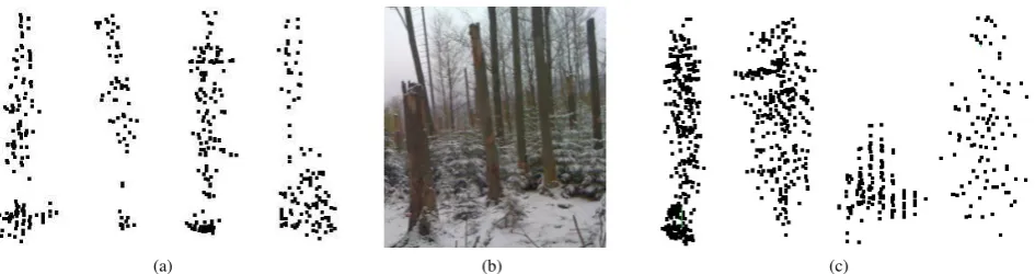
Figure 1: Examples of ALS point clouds of dead trunks (a) and other forest structures (c). The other objects include slender trees, small bushes/ground vegetation, and trees that were poorly captured in the point cloud due to low point density. (b) shows an optical image of several dead trunks surrounded by small trees near the ground.
class of interest. In particular, parts of the axis where no relevant information is usually present can be excluded from contributing anything to the descriptor, preventing the introduction of clutter. Also, the length, radius and number of subdivisions of each local cylindrical neighborhood is independent from all other parts of the descriptor. Due to the required existence of a principal axis, the FSC is primarily applicable to elongated objects such as trees, logs, lamp poles, traffic signs etc. Our choice of the SC over the aforementioned surface descriptors (SI, PFH) stems from the as-sumption that the objects’ surface reflected in the point cloud may be noisy and incomplete, resulting in an inability to reliably es-timate the normals. Therefore, the volumetric nature of the SC makes it more suitable for representing the target objects in our scenario. Moreover, the higher number of degrees of freedom (dimensions of the bin divisions) endows the SC with more flexi-bility to tailor a feature set appropriate for a specific classification problem. Another argument in favor of the SC is its successful application in the related task of detecting fallen tree segments (Polewski et al., 2014, 2015). The high flexibility of the new FSC descriptor comes at a cost of a significantly bigger parame-ter space, because not only the radii and lengths of the cylindrical neighborhoods, but also theirstructure, i.e. counts, arrangement along the axis, number of embedded cylinders, must be deter-mined through optimization. To tackle this problem, we apply a genetic algorithm (GA) (Goldberg, 1989), a powerful meta-heuristic optimization method which maintains a population of solutions (’individuals’) and attempts toevolvethem towards an optimal solution by promoting high-quality individuals and by re-combining existing individuals into new ones through cross-over and mutation, in analogy to an evolutionary process. Among their many successful applications in various fields, GAs have been used to find the optimal neighborhood sizes for features obtained from the 3D covariance matrix (Waldhauser et al., 2014), as well as the optimal parameters of a 3D shape descriptor based on two cylindrical neighborhoods (Wegrzyn and Alexandre, 2013).
The issue of selecting an optimal neighborhood size for feature construction in point clouds has received considerable attention within the remote sensing community. Weinmann et al. (2014) propose an eigenentropy-based scale selection for spherical point neighborhoods. Blomley et al. (2014) analyze the influence of scale on classification accuracy for cylindrical neighborhoods. The authors employ the aforementioned originallyglobalShape Distributions to describelocalpoint neighborhoods using an adap-tive histogram binning scheme. However, it should be noted that these and other proposed approaches are defined at the individ-ual pointlevel, whereas our method aims at describing the entire
objectby concatenating local descriptors of varying complexity.
We test the proposed shape descriptor in the context of the task of detecting standing dead tree trunks. Information about the
dis-tribution of dead wood in forests is of interest in environmental sciences because of its role in biodiversity of plant and animal species (Stokland et al., 2012) and nutrient cycles (Siitonen et al., 2000). Due to their small cross-section area, dead trunks are hardly visible on aerial imagery and hence cannot be reliably de-tected from this data source. Therefore, full 3D information pro-vided by LiDAR point clouds is advantageous for this scenario. The dead trunks exhibit some variability in appearance due to residual branches and the potential presence of ground vegeta-tion. A further difficulty is their resemblance to slimmer trees (see Figure 1).
The rest of this paper is structured as follows: in Section 2. we describe the overall object detection pipeline, including input data requirements. Section 3. introduces the new Free Shape Context descriptor in detail and outlines the Genetic Algorithm approach used for optimizing the FSC parameters. Section 4. describes the study area, experiments and evaluation strategy. The results are presented and discussed in Section 5. Finally, the conclusions are stated in Section 6.
2. OVERALL STRATEGY
The input to our detection pipeline consists of ALS point clouds given in the form of 3D coordinate sets. Both discrete return and full waveform systems may be used, however the point den-sity should be sufficient for distinguishing the objects of interest within the point clouds. Our method is based purely on geomet-ric features and does attempt to utilize radiometgeomet-ric information. The entire processing pipeline is depicted in Figure 2. In the first step, the point cloud is partitioned into subsets which represent single objects. We view the partitioning step as an external pro-cedure and do not focus on it in this study. It can be carried out using any appropriate clustering method. In particular, we use the Normalized-Cut based approach by Reitberger et al. (2009). For the case when the target objects are well separated in the scene, a connected component search such as the pre-processing step de-scribed by Velizhev et al. (2012) may also be used. Each point cluster is then processed individually as an object candidate. We first compute the axis of the point cloud using a Sample Con-sensus method. The object-level features are then calculated and each candidate object is labeled as either target class or non-class. In order to optimize the discriminative power of the features, we also require that a set of objects (outputs from the clustering step) labeled as either class or non-class be provided to serve as train-ing data.
Calculating object axis
cluster-Figure 2: Overview of dead trunk detection pipeline.
ing step is likely to produce imperfect partitions, the presence of clutter and/or parts of other objects is expected within the point cloud. For this reason, we apply an estimation method from the Random Sample Consensus (SAC) family to calculate the axis. As opposed to fitting a model to the entire input data, SAC meth-ods aim at improving robustness to outliers by randomly generat-ing model hypotheses and evaluatgenerat-ing how well they fitsubsetsof the data according to a scoring scheme. The score corresponds to the total fit error and hence the lowest-scoring model is returned as the fitting result. The error is usually a function of the num-ber of inlier points within a fixed distance from the model and also of the quality-of-fit to the inliers. Since we wish to maxi-mize both of these possibly contradictory criteria simultaneously, it is necessary to define a tradeoff between them in order to ob-tain a single criterion function for optimization. Specifically, we make use of the M-estimator SAC variation (Torr and Zisserman, 2000) with a line model, cylindrical neighborhood with radius
rsacand point-to-line perpendicular distanced(·,·). The error of line modelLon point setP is defined as follows:
CP(L) =
X
p∈P
ρ(d2(p, L)), ρ(d2) = (
d2
d2
< r2 sac
r2 sac d
2 ≥r2
sac (1)
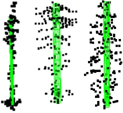
We additionally introduce a constraint on the maximum angular deviationαdev of the candidate line models from the world Z coordinate axis to account for the phenomenon of gravitropism in trees. A sample result of the calculated axes for several point clouds is depicted by Figure 3.
Figure 3: Axes of point clouds determined by Sample Consensus.
3. SHAPE DESCRIPTORS
3.1 3D Shape Contexts
Originally introduced by Frome et al. (2004) as a local shape de-scriptor of surface patches, the 3D Shape Context (SC) attempts to capture the shape distribution inside a volume of a point cloud by subdividing the volume into bins along 3 dimensions and cre-ating a histogram by counting the points in each bin. We replace the original spherical neighborhood centered on a point with a cylindrical neighborhood around an axis. The cylinder is divided along the axial, radial and angular dimensions (see Figure 4). Note that the angular division may cause the SC to lose its ro-tational invariance, since two rotated copies of the same point cloud with the same axis may in general produce different his-togram signatures. To remedy this, a method of defining the common0◦orientation is required. An alternative would be to augment the training set with rotated copies of each labeled ex-ample. In this work, for the sake of simplicity we refrain from dividing the cylinder along the angular dimension and thus retain the invariance w.r.t. rotation. The radial subdivisions follow an exponential law of the form: ri =r0riB, where the base radius
r0and the exponential baserBare user-defined parameters. The remaining parameters consist of the SC’s lengthl, the number of axial divisionsnL, and the outer radiusrmax.
Figure 4: Cylindrical shape context around axis. Center: side view. Right: top view. Only single angular category shown.
3.2 Free Shape Contexts
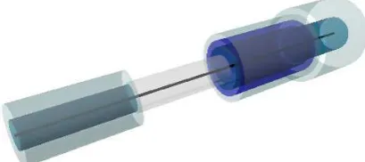
The standard Shape Context defined in Sec. 3.1 has a uniform structure. However, for a specific detection task, it is unlikely that discriminative information is evenly distributed along the ob-ject axis. In particular, some parts may be heavily affected by clutter, which renders them useless as a source of distinctive fea-tures. Furthermore, for the parts which are relevant, the optimal neighborhood may significantly vary in size. Based on these two intuitions, we propose a new shape descriptor, the Free Shape Context (FSC). The FSC is essentially a stack of cylindrical vol-umes arranged around the axis. This can be viewed as a sequence of adjacent standard SCs which are divided only along the radial dimension, i.e. potentially contain embedded cylinders of smaller radii (see Figure 5). The lengths and radii of the constituent SCs are unrelated and may be adjusted independently. Additionally, every cylinder has an activity state which controls whether the associated histogram bin is allowed to emit a feature to the final descriptor. Inactive cylinders can be regarded as buffer elements -they only define the structure of the FSC without affecting feature values. The FSC is parameterized by the ordered sequence of the member SCs’ parameters. Each such SC is in turn described by its length and sequence of cylinder radii along with their corre-sponding active states.
Figure 5: A Free Shape Context. Gray cylinder near middle is inactive - it will not contribute to the shape histogram.
space. To analyze the parameter space, we first introduce some notation. LetNR, NLbe the number of quantized radius and length configurations, respectively, that can be examined with a reasonable computational effort. We then have that for an FSC consisting of a single SC with a single cylinder, the number of configurations is2NRNL. The factor2arises from the two pos-sible activity states. If we add a new cylinder to the SC, we can set the new radius to any other of theNR values, assign it an active or passive state and combine it with any previous config-uration, resulting in22 NR
2
NLoptions. Following this line of reasoning, the number of configurations for an FSC consisting of one SC withicylinders is: C1,i = 2i NiR
NL. Letnr de-note the maximal number of radial bins. We can express the total number of FSC configurations consisting ofk SCs usingC1,i:
Ck = (C1,1+. . .+C1,nr)
k. This expression is dominated by
the term{2nr NR
nr
NL}k. It can be easily verified that even for a coarse quantization of the radii and lengths and a small number of SCs, the computational complexity renders any exact or even grid search approach infeasible.
3.2.2 Approximate optimization It is possible to alleviate the computational burden by making two simplifying assumptions. The first assumption states that the problem of finding the most discriminative FSC exhibits the optimal substructure property. In practice this means that if the best FSCfof lengthLcontains its last shape contextsfrom positionsDtoLalong the axis, then the FSC obtained by removingsfromfmust be the most discrimi-native FSC of lengthD. The second assumption recasts this re-quirement in the context of cylinder radii within a single SC. The optimal substructure premise gives rise to a dynamic program-ming strategy for calculating the optimal FSC. LetWk,j denote the best score of ak-component FSC of (quantized) lengthj, and
Pk,jthe corresponding FSC parameters. Also, letVk,j(P, l)be the smallest error of an FSC formed by combining the parameters
Pwith a new SC consisting ofkcylinders with a total (external) radiusjand lengthl. LetSP,lk,jdenote this optimal SC, andcr- a cylinder with radiusr. The minimum cost can then be calculated:
Wk,j= min{Wk,j−1,min
l,u,vVu,v(Pk−
1,j−l, l)} (2)
Vk,j(P, l) = min{Vk,j−1(P, l),min
r E(P⊕[S P,l
k−1,j−r∪cj])} In the above,⊕denotes appending an SC at the end of an FSC, andE(·)is the evaluation function (e.g. classification error).
3.3 Evolving optimal FSC parameters
Due to the size of the parameter space of the FSC, it is unlikely that any approach which attempts to sample parameters in equal intervals (such as the dynamic algorithm described in Sec. 3.2.2) will attain a near-optimal solution. The parameter space is usu-ally highly heterogeneous, with small isolated regions of high-quality solutions. Also, the optimal substructure assumptions
may not be valid. Therefore, it appears more beneficial to in-stead apply an optimization strategy which is capable of dedi-cating more effort to the exploration of promising regions of the solution space at the expense of omitting its weaker parts, thereby making a better use of the allocated resources. One such method is the Genetic Algorithm, a biologically-inspired meta-heuristic which has been successfully applied to the optimization of multi-ple problems in science and engineering.
Genetic algorithms As a representative of evolutionary com-putation methods, Genetic Algorithms (Goldberg, 1989) are an optimization technique which attempts to mimic an evolutionary process. In the language of the biological metaphor, solutions to the problem of interest are referred to asindividualsand are en-coded using agenetic representation. The value of the optimized functionf associated with a solution is called thefitness func-tionof the individual. The genetic algorithm acts on apopulation
of individuals by iteratively selecting the best elements based on their fitness and subsequently recombining them to create a new generation of individuals. The recombination usually consists of two parts: mutation and crossover. Mutation is a unary opera-tor which randomly alters small parts of the target individual’s genome. Crossover is an operator acting on a pair of individu-als (’parents’) with the purpose of randomly exchanging parts of their genomes. The iteration is repeated until a convergence cri-terion is met. It is expected that in the course of evolution, the individuals will gradually improve their fitness until a (local or global) extremum of the fitness function is attained.
3.3.1 FSC genotype representation We use a variable-length, structured genetic representationG(c)of the Free Shape Context
c. At the top level, the genome is an ordered sequence of the constituent SCs’ sub-genomes:G(c) = (G(sc1), . . . , G(scN)). Each sub-genomeG(sck) = (lk,([rk,i, ak,i])i=1..nk)is
com-posed of the lengthland list of thenkcylinder radiirand active statesa. We make the distinction betweenstructural parameters, which describe the number of SCs, the number of radii within each SC as well as the active state of each cylinder, andsize pa-rameters, which encode the cylinder lengths and radii.
3.3.2 Mutation For the structural parameters, we employ a simple mutation scheme which randomly adds and removes SCs from the FSC, adds and removes cylinders from a single SC, or flips the active state. All of these events occur with a small prob-abilitypm,1. For the size parameters, a relative mutation strategy is used. A random numberκis drawn from a zero-mean normal distribution with standard deviationσm∈ (0; 1), and the target parameterpis updated according to: p←p(1 +κ). This mu-tation takes place with a probabilitypm,2> pm,1. The mutation rates for the structural and size parameters are distinct because we want the evolutionary process to spend sufficient effort exam-ining the size parameters for a given structure. This is motivated by the fact that the number of structural configurations is small compared to the number of length/radius configurations.
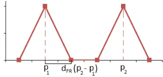
distribution on the output value, with modes located atp1andp2 (Figure 6). Large values ofdF Rlead to introducing more diver-sity into the population, whereas small values benefit the protec-tion of good existing soluprotec-tions.
Figure 6: Bi-triangular output distribution induced by Fuzzy Re-combination operator.
3.3.4 Fitness function The evolution of the Free Shape Con-texts is driven by their overall classification performance on a set of labeled objects (point clouds). In particular, we do not parti-tion the labeled pool into training and test sets, but instead apply a cross-validation scheme for calculating the classification error. It is important that the error measure be deterministic in the sense of always obtaining the same error value upon repeated calcu-lation for the same individual. Otherwise, the evolution could be promoting random constellations of training vs. test set parti-tions which lead to lower errors at the expense of true discrimina-tive performance. For this reason, we apply leave-one-out cross-validation which is free from any randomness.
3.4 Adaptive tuning of GA parameters
A key issue in a successful application of a GA to a specific do-main is whether the GA can attain a balance betweenexploitation
andexploration. The former can be understood as the capability to thoroughly search promising regions of solution space, thereby ’exploiting’ the neighborhood of high-quality solutions. The lat-ter is associated with a broader strategy of ’exploring’ all relevant parts of the solution space as opposed to the evolutionary pro-cess getting stuck in a local optimum. The recombination meta-parameters (e.g.pm,1,pm,2,dF R) have a decisive influence on the GA’s dynamic behavior (Herrera and Lozano, 2001). On the other hand, manually setting these meta-parameters is a non-trivial task usually accomplished through resource-expensive trial-and-error procedures. For these reasons, methods have been developed which are able to adaptively change the meta-parameter settings during the evolution, based on feedback from the evolutionary process. We take an approach inspired by the contributions of Herrera and Lozano (2001) as well as Lee and Takagi (1993). The principal idea is to utilize a fuzzy logic controller (FLC) to calculate the FR widthdF Rseparately for each application of the FR crossover operator, based on the fitness of the parents and the overall diversity of the entire population. The processing pipeline of the GA augmented with the FLC is shown in Figure 7. The fuzzy rules comprising the optimal FLC are themselves found us-ing a genetic algorithm. Specifically, a two-tier evolution scheme is set up. At the top level, a small population of FLCs is evolved. Each FLCcis evaluated by executing an instance of the Free Shape Context evolution (bottom level) and lettingccontrol the FR width. The fitness of c is the offline performance of the bottom-level GA, i.e. the best fitness of any individual found up to the current iteration, averaged over all iterations.
3.4.1 Fuzzy inference Fuzzy logic (Klir and Yuan, 1995) is an extension of Boolean logic to multi-valued domains. As op-posed to crisp Boolean values of true and false, a fuzzy variable may assume any continuous value from the interval[0; 1]. This value represents a subjective degree of belief that a proposition is
Figure 7: Overview of GA for finding best FSC parameters. FLC adapts the FR width for crossover using 9 fuzzy rules based on the population diversity and the parents’ fitness (fit1, fit2).
true, with0,1representing absolute falseness and absolute truth, respectively. This formulation makes fuzzy logic appropriate for modeling uncertain or vague relationships between variables. To perform fuzzy inference, an additional level of abstraction in the form of linguistic variables and fuzzy sets is defined. A linguis-tic variable represents any quantity that is of interest in the ap-plication (e.g. ’temperature’), along with its enumerated possi-ble values (e.g. ’high’,’medium’,’low’). Each variapossi-ble level is associated with a fuzzy set, which is in turn defined by a fuzzy membership functionµ(x)∈[0; 1]. Based on linguistic variables
X, Y, Zwith levelsa, b, c, fuzzy rules may be defined:
IF X IS a AND Y IS b THEN Z IS c
The application of fuzzy rules requires defining a fuzzy ’and’ op-erator, implication function, rule output aggregation and defuzzi-fication method for converting the fuzzy rule results into a crisp number.
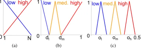
3.4.2 Fuzzy logic controller for GA The FLC responsible for setting the FR width uses three linguistic variables as input. The first two are the ranks (ordinal numbers) of each parent’s fitness within the entire population. The two fitness variables assume the values ’high’ and ’low’. Their corresponding fuzzy membership functions are fixed (see Figure 8(a)). Following Lee and Takagi (1993), we also introduce the population diversity as an input variable with three levels: ’high’, ’medium’, and ’low’, to enable the FLC to employ different strategies depending on the current stage of the evolution. The fuzzy membership functions of the diversity levels are parameterized by the locationsdland
dm(Figure 8(b)). Finally, the output variable (FR width) also as-sumes the three levels ’high’, ’medium’, and ’low’, with fuzzy membership functions defined by the parametersol,om, andoh (Figure 8(c)). For each diversity level, three decision rules are defined which assign an FR width level for every combination of parent fitness ranks (the high-low and low-high cases are sym-metric), yielding a total of 9 rules. The output levels of all rules are evolved together with the 5 fuzzy membership location pa-rameters to produce the FLC whose control actions lead the em-bedded Free Shape Context evolution to attain the best offline performance.
1
Figure 8: Fuzzy membership functions of (a) fitness ranks (N -population size) (b) -population diversity, (c) output variable.
is normalized on the interval[0; 1]and is taken as the average distance between the member SCs ofc1andc2at corresponding positions. For two SCss1, s2, their distance is in turn defined as
1−Vi/V, whereV is the maximum ofs1ands2’s outer cylin-der volumes, andViis the sum of the intersection volumes of the corresponding cylindrical bins ins1ands2. If the number of SCs withinc1 andc2 is not equal, each excess SC without a corre-sponding element is regarded as having the maximum distance of 1 (consistent with an intersection volume of 0).
4. EXPERIMENTS
4.1 ALS data
For testing the proposed methodology, we used a 1x1 km2plot lo-cated in the Bavarian Forest National Park (49◦3′19′′
N,13◦12′9′′ E), which is situated in South-Eastern Germany along the border to the Czech Republic. The study was performed in the mountain mixed forests zone consisting mostly of Norway spruce (Picea abies) and European beech (Fagus sylvatica). The dead wood originated from an outbreak of the spruce bark beetle (Ips ty-pographus) in recent years. The airborne full waveform ALS data were acquired using a Riegl LMS-680i scanner in July 2012 with a nominal point density of 30-40 points/m2and pulse rate of 266 kHz. The flying altitude of 650 m led to a footprint size of 32 cm.
4.2 Reference data
To create a data set for assessing the performance of each feature family, we first performed the segmentation into individual trees (Reitberger et al., 2009). We then manually selected and labeled a total of 285 objects to serve as the basis for our study, of which 56% were living trees and 44% were dead trunks. The average point counts in the segmented point clouds of the objects were 340 and 208 respectively for living trees and dead trunks. The selection criterion was associated with ensuring a possibly broad coverage of both classes’ appearance ranges within the ALS point cloud. The labeling was done based on visual inspection of each object’s point subset.
4.3 Detailed experiments
We designed two experiments to attain detailed insight into the performance of the proposed Free Shape Context features com-pared to other competing feature families in the context of our classification problem. In all calculations, we used the same in-put data, classification model (logistic regression), determinis-tic evaluation criterion (leave-one-out cross validation), and pre-calculated object axes, therefore the differences between the de-tection rates can solely be attributed to the features themselves. A value of2◦
was used for the angular deviation thresholdαdev.
4.3.1 Comparison of feature families In the first experiment, we compare the performances of Free Shape Contexts, standard
(uniform structure) Shape Contexts, and features based on eigen-values of the covariance matrix (referred to as CE). To under-stand what part of the potential gain in classification accuracy is associated with the features as opposed to being merely a result of applying a better optimization strategy (genetic algorithm vs. grid search), we tested each feature family in two configurations. The first variation uses parameters optimized by grid search (in case of FSC the dynamic algorithm described in Sec. 3.2.2), while the second configuration is based on GA parameter optimization. In all GA-based experiments, we used the same population size (1000) and generation count (150) as well as selection mecha-nism (size 5 tournament selection). Because the GA optimiza-tion result is non-deterministic, we repeated the experiments 15 times from random initializations. For FSC, the maximum al-lowed number of member SCs was 12, each with up to 5 radial bins. The meta-parameter settings (Sec. 3.3) were:pm,1= 0.03,
pm,2 = 0.15,σm = 0.1,pF R = 0.6. In this experiment, the FR width was fixed at a value ofdF R = 0.05. This value was chosen empirically from a small set of discrete levels based on the results of preliminary experiments with smaller population sizes and generation counts. For the evolution of standard SCs, we applied a vector of 5 real numbers representing the param-etersr0,rB,l,nl,rmaxas the SC’s genotype, with two-point crossover and Gaussian mutation (such as the size parameter mu-tation in Sec. 3.3.2). Finally, for the CE features, we defined a simple variation of the Bag-of-Features model (Toldo et al., 2009). For each point within the input point cloud, we calcu-late the values of the 8 CE features defined in (Weinmann et al., 2014) (Table 1). We then partition the domain of each featurei
intobiequidistant bins. Each bin defines a ’visual word’ for the associated attribute. The descriptor of the entire scene consists of the decorrelated, concatenated histograms of visual word counts for each feature over all points within the scene. The parameters of this model are the numbers of feature partitionsbias well as the common neighborhood radius for calculating the covariance matrix around each point. Note that a value of 0 partitions causes the feature to be omitted from analysis, which enables a simulta-neous feature selection. We utilize a similar strategy for genetic representation and recombination as was the case with standard SC evolution. The grid search/dynamic algorithm approximation strategies were carried out with a number of inspected configura-tions greater than or equal to the number of individuals processed in a single GA execution (1000 * 150 = 150000).
5. RESULTS AND DISCUSSION
5.1 Comparison of feature families
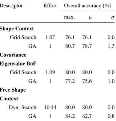
Table 1 summarizes the overall classification results for all 6 tested combinations of feature families and optimization algorithms. The computational effort is measured in units equal to the number of evaluations of individuals in a single GA run, i.e. 150000, with 1 unit corresponding to about 6 hours of absolute processing time on a quad-core IntelR
XeonR
processor with a base frequency of 3.7 GHz. In case of the two SC-based feature types, the ge-netic algorithm is able to outperform the grid search/dynamic al-gorithm by up to 4.6 percentage points (pp), using less parameter configuration evaluations. Also, in case of the Free Shape Con-texts, the dynamic algorithm is not able to find a solution com-parable to one obtained through GA despite a tenfold increase in the used computational resources. This is an expected result due to the discussed high computational complexity of optimiz-ing the FSC parameters (Sec. 3.2.1). For the sake of fairness, it should be noted that because they are stochastic in nature, ge-netic algorithms do not always converge to the best found solu-tion. In fact, we observed that for all three feature types, out of 15 runs with random initializations, the best solution was only obtained 1-2 times. This emphasizes the difficulty in finding an optimal set of GA meta-parameters which reliably leads to convergence under different initializations. On the other hand, even the mean classification accuracies averaged over all restarts outperform their counterparts from grid search for SC and FSC. Interestingly, the GA seems to fail as an optimizer of CE
param-Descriptor Effort Overall accuracy [%]
max. µ σ
Shape Context
Grid Search 1.07 76.1 76.1 0.0
GA 1 80.7 78.7 1.3
Covariance
Eigenvalue BoF
Grid Search 1.09 80.0 80.0 0.0
GA 1 77.2 75.6 1.0
Free Shape
Context
Dyn. Search 10.44 80.0 80.0 0.0
GA 1 84.2 82.7 0.8
Table 1: Evaluation results for considered features w.r.t. clas-sification accuracy. Workload reflects the number of evaluated parameter sets (1 = number of evaluations in a single GA run).
eters, its best found solution lagging by 2.8 pp behind the grid search result. We hypothesize that this may be due to the CE parameters consisting mostly of integers (numbers of feature di-visions) as opposed to the SC and FSC parameters being mostly reals (cylinder lengths and radii). This makes it harder for the evolutionary process to find a gradient of the optimized function w.r.t. the more discretized parameter space. Perhaps a genetic representation or recombination method more suitable for inte-ger variables could remedy this problem. In terms of the best-performing solution, the CE features appear to be inferior to both SC and FSC. This indicates that the point density afforded by ALS point clouds is not sufficient so as to support discriminating between different surface types on a scale finer than several me-ters. This claim is further supported by the fact that the optimal
CE performance arose from a neighborhood radius of 4.4 m for the covariance matrix calculation (from an available interval of 0.1-5 m), which implies that the no meaningful way to utilize in-formation based on smaller neighborhoods could be found. The proposed Free Shape Context-based features have delivered the best performance. For average quality of the GA-optimized so-lutions, FSC outperforms SC by 4 pp and CE by 7.1 pp, whereas in case of the best found solution, the respective gains are 3.5 pp and 4.2 pp. Regarding the feature counts associated with each descriptor, the best FSC feature set had a cardinality of 10, equal-ing the correspondequal-ing count for CE and lyequal-ing significantly below the SC-related count of 30. Combined with the superior perfor-mance, this suggests that, compared to its competitors, the FSC descriptor was able achieve a better balance between finding the relevant, discriminative parts of the target objects and omitting non-informative parts. To investigate the statistical significance of the performance differences, we used the one-tailed binomial test. We regard the outcome of the labeling ofN objects by a classifier with accuracypas a random variable with a binomial distributionB(N, p). In particular, for the pair FSC-CE, we test if the result of 240 successfully classified objects is likely to have arisen from a distributionB(285,0.8). The obtainedp-value is 0.04, so the difference is significant at a level of 0.05. Similarly, for the pair FSC-SC, thep-value lies at 0.07. In contrast, the dif-ference between SC and CE is considerably less significant with ap-value of 0.42.
5.2 Evaluation of FLC for adaptive control
optimal solution in any of the 25 random retries, which means that the FLC’s design was tightly coupled with initial population which it was exclusively optimized on. Therefore, its overall gen-eralization capability is poor.
Finally, the implicit assumption about the correctness of the cal-culated object axis should be addressed. For the dead trunks, the SAC-based axis calculation method usually succeeds since the tree crown is missing and many stem hits are available. However, problematic cases may arise in the presence of dense ground veg-etation and an asymmetric residual branch structure, leading to an erroneous axis. For living trees, this is even more of a concern. In this study, we did not investigate the axis quality and its influence on the classification accuracy, but the fact that both axis-based de-scriptors outperformed the axis-independent covariance features indicates some level of robustness to axis displacement.
6. CONCLUSIONS
This paper introduced a new kind of shape descriptor for clas-sification tasks in sparse point clouds, the Free Shape Context (FSC), which is based on a sequence of cylindrical 3D Shape Contexts organized around a common axis. We have shown that owing to its increased number of degrees of freedom, the FSC can exploit characteristic regions of the target objects while regarding cluttered or non-informative regions, yielding good dis-criminative power and simultaneously keeping the cardinality of the feature set at low levels. Specifically, the proposed FSC de-scriptor was able to outperform, in a statistically significant man-ner, a simple Bag-of-Features model based on covariance matrix eigenvalue features, and a standard 3D Shape Context descrip-tor. Our results show that the FSC can be a viable alternative to local features based on eigenvalues of the point neighborhood’s covariance matrix for inference tasks in ALS point clouds. The higher number of degrees of freedom leads to an increased com-putational complexity, which prevents using exact or grid search approaches for optimizing the FSC parameters. We have demon-strated that a genetic algorithm (GA) is suitable for this task. Also, the successful application of a Fuzzy Logic Controller for adapting the Fuzzy Recombination width meta-parameter con-firms previous results from the field of evolutionary computation showing that the meta-parameter selection may be partially au-tomatized by combining GA with fuzzy logic. In the future, it would be interesting to confirm the FSC’s discriminative capa-bilities on other kinds of remote sensing data. Also, the FSC’s expressive power could benefit from introducing subdivisions in the angular dimension, although this would require a strategy for ensuring rotational invariance around the axis. Finally, to ease the computational burden of finding the optimal FSC parameters, in-stead of directly estimating the classification error induced by an FSC, an approximate quality assessment scheme could be used.
REFERENCES
Blomley, R., Weinmann, M., Leitloff, J. and Jutzi, B., 2014. Shape distribution features for point cloud analysis - a geometric histogram approach on multiple scales.ISPRS Ann. Photogramm. Remote Sens. Spatial Inf. Sci.II-3, pp. 9–16.
Frome, A., Huber, D., Kolluri, R., B¨ulow, T. and Malik, J., 2004. Recognizing Objects in Range Data Using Regional Point De-scriptors. In:Proceedings of the European Conference on Com-puter Vision (ECCV).
Goldberg, D. E., 1989. Genetic Algorithms in Search, Optimiza-tion and Machine Learning. 1st edn, Addison-Wesley Longman Publishing Co., Inc., Boston, MA, USA.
Herrera, F. and Lozano, M., 2001. Adaptive genetic operators based on coevolution with fuzzy behaviors. IEEE Trans. Evolut. Comput.5(2), pp. 149–165.
Johnson, A. and Hebert, M., 1999. Using spin images for efficient object recognition in cluttered 3D scenes. IEEE Trans. Pattern Anal.21(5), pp. 433–449.
Klir, G. J. and Yuan, B., 1995. Fuzzy Sets and Fuzzy Logic: The-ory and Applications. Prentice-Hall, Upper Saddle River, USA. Lee, M. A. and Takagi, H., 1993. Dynamic control of genetic al-gorithms using fuzzy logic techniques. In:Proceedings of the 5th International Conference on Genetic Algorithms, Morgan Kauf-mann Publishers Inc., San Francisco, CA, USA, pp. 76–83. Mallet, C., Bretar, F., Roux, M., Soergel, U. and Heipke, C., 2011. Relevance assessment of full-waveform lidar data for urban area classification. ISPRS J. Photogramm. Remote Sens.66(6), pp. S71 – S84.
Osada, R., Funkhouser, T., Chazelle, B. and Dobkin, D., 2002. Shape distributions.ACM Trans. Graph.21(4), pp. 807–832. Polewski, P., Yao, W., Heurich, M., Krzystek, P. and Stilla, U., 2014. Detection of fallen trees in ALS point clouds by learn-ing the Normalized Cut similarity function from simulated sam-ples. ISPRS Ann. Photogramm. Remote Sens. Spatial Inf. Sci.
II-3, pp. 111–118.
Polewski, P., Yao, W., Heurich, M., Krzystek, P. and Stilla, U., 2015. Detection of fallen trees in ALS point clouds using a Normalized Cut approach trained by simulation. ISPRS J. Pho-togramm. Remote Sens.105, pp. 252 – 271.
Reitberger, J., Schn¨orr, C., Krzystek, P. and Stilla, U., 2009. 3D segmentation of single trees exploiting full waveform LIDAR data.ISPRS J. Photogramm. Remote Sens.64(6), pp. 561 – 574. Rusu, R., Marton, Z., Blodow, N. and Beetz, M., 2008. Learn-ing informative point classes for the acquisition of object model maps. In:10th International Conference on Control, Automation, Robotics and Vision, pp. 643–650.
Saupe, D. and Vranic, D., 2001. 3D model retrieval with spherical harmonics and moments. In: B. Radig and S. Florczyk (eds),
Pattern Recognition, Lecture Notes in Computer Science, Vol. 2191, Springer Berlin Heidelberg, pp. 392–397.
Siitonen, J., Martikainen, P., Punttila, P. and Rauh, J., 2000. Coarse woody debris and stand characteristics in mature managed and old-growth boreal mesic forests in southern Finland. Forest Ecol. Manag.128(3), pp. 211 – 225.
Stokland, J. N., Siitonen, J. and Jonsson, B. G., 2012. Biodi-versity in Dead Wood. Cambridge UniBiodi-versity Press. Cambridge Books Online.
Toldo, R., Castellani, U. and Fusiello, A., 2009. A Bag of Words Approach for 3D Object Categorization. In: A. Gagalowicz and W. Philips (eds), Computer Vision/Computer Graphics Collab-oration Techniques, Lecture Notes in Computer Science, Vol. 5496, Springer Berlin Heidelberg, pp. 116–127.
Torr, P. and Zisserman, A., 2000. Mlesac: A new robust estimator with application to estimating image geometry.Computer Vision and Image Understanding78(1), pp. 138 – 156.
Velizhev, A., Shapovalov, R. and Schindler, K., 2012. Implicit shape models for object detection in 3D point clouds.ISPRS Ann. Photogramm. Remote Sens. Spatial Inf. Sci.I-3, pp. 179–184. Waldhauser, C., Hochreiter, R., Otepka, J., Pfeifer, N., Ghuffar, S., Korzeniowska, K. and Wagner, G., 2014. Automated Classi-fication of Airborne Laser Scanning Point Clouds. In: S. Koziel, L. Leifsson and X.-S. Yang (eds),Solving Computationally Ex-pensive Engineering Problems, Springer Proceedings in Mathe-matics & Statistics, Vol. 97, Springer, pp. 269–292.
Wegrzyn, D. and Alexandre, L., 2013. A Genetic Algorithm-Evolved 3D Point Cloud Descriptor. In: J. Ruiz-Shulcloper and G. Sanniti di Baja (eds),Progress in Pattern Recognition, Image Analysis, Computer Vision, and Applications, Lecture Notes in Computer Science, Vol. 8258, Springer, pp. 92–99.