INVESTIGATIONS ON THE POSSIBILITIES OF MONITORING COASTAL CHANGES
INCLUDING SHALLOW UNDER WATER AREAS WITH UAS PHOTO BATHMETRY
G.J. Grenzdörffer a, M. Naumann a
a Rostock University, Chair for Geodesy and Geoinformatics, J.-v.-Liebig Weg 6, Rostock, Germany- [goerres.grenzdoerffer], [matthias.naumann]@uni-rostock.de
Commission I, ICWG I/Vb
KEY WORDS: UAS-Photogrammetry, 3D-Point Cloud, photo bathymetry
ABSTRACT: UAS become a very valuable tool for coastal morphology. Not only for mapping but also for change detection and a better understanding of processes along and across the shore. This contribution investigates the possibilities of UAS to determine the water depth in clear shallow waters by means of the so called "photo bathymetry". From the results of several test flights it became clear that three factors influence the ability and the accuracy of bathymetric sea floor measurements. Firstly, weather conditions. Sunny weather is not always good. Due to the high image resolution the sunlight gets focussed even in very small waves causing moving patterns on shallow grounds with high reflection properties, such as sand. This effect invisible under overcast weather conditions. Waves, may also introduce problems and mismatches. Secondly the quality and the accuracy of the georeferencing with SFM algorithms. As multi image key point matching will not work over water, the proposed approach will only work for projects closely to the coastline with enough control on the land. Thirdly the software used and the intensity of post processing and filtering. Refraction correction and the final interpolation of the point cloud into a DTM are the last steps. If everything is done appropriately, accuracies in the bathymetry in the range of 10 – 50 cm, depending on the water depth are possible.
1 INTRODUCTION
Constructions in coastal environments, such as levees, harbors etc. require precise 3D-topographic information. Also for monitoring the coastal morphology, accurate and affordable data is necessary to improve the knowledge about morphological processes and topographical evolution. Accurate topographic / bathymetric measurements are also required to monitor related sediment transport and morphological changes. Morphological changes occur on one hand more or less continuously with a small rate of change and on the other hand drastically during an extreme event, such a major storm or an extreme tide. Therefore, it is important to improve the temporal frequency of data acquisition in order to determine the magnitude of change for a given period, Mancini et al. 2015. The computation of Digital Elevation Models of Difference (DoDs), derived by comparing DEMs from two or more surveys, has become a standard methodology to detect the sediment movement trends and quantify volumes of cut and fill over events and longer timescales.
Yet shallow coastal water regions with depths of 0 m to 2 m are particularly difficult to measure, because these areas are not accessible for vessels in many cases. Thus, data of these regions are often not very accurate and sometimes missing, although they are needed for many of the above mentioned applications related to coastal protection and coastal zone management. Unmanned Aerial Systems (UAS) image surveys appear as a perfect solution for coastal monitoring, as they are able to derive topographic information on land and maybe also under water.
Several studies, e.g. Flener et al, 2012. Javernick et al., 2014, Williams et al., 2014, Woodget et al., 2015 used UAS images successfully at river systems and derived the water depth with an optical–empirical bathymetric mapping approach with decimetre accuracy. For a successful implementation of this approach the observed water colour must be related to the
attenuation of the river bottom reflection caused be the depth of the water. Thus this approach only works well if sufficient bathymetric reference data is available, the river bottom is homogeneous and the water has a constant low turbidity, e.g. sandy or gravel river beds. This is not necessarily the case in coastal environments, with varying grounds. In coastal areas more satellite based bathymetry is commonly used, e.g. Needham & Hartmann, 2013.
Laser bathymetry is another established method of airborne measurements of the sea bottom of shallow coastal areas. Thus, it is an alternative technique compared to conventional (multibeam) echo sounder data of ships, which is even more time consuming and costly, e.g. Guenther et al., 2000, Costa et al., 2009. The LiDAR system uses two lasers, a green laser which can penetrate the water column and an infrared laser, which is reflected at the water surface. The depth is subsequently determined from the two-way runtime between the water surface and reflections from the solid ground underneath. The visibility of the water is the main limiting factor for the achievable depth measurements. As a measure for visibility the term “secchi” is used, where one secchi is the maximum depth of which the human eye can make out a white disk in the water. Bathymetric LiDAR systems today work from one to about three secchi depths. Significant depth readings of up to 6 m are reported for the Baltic coast, Niemeyer et al., 2014.
multi-ray photogrammetry additional problems arise, e.g. Jordt-Sedlazeck & Koch (2013).
1.1 Workflow for UAS-photo bathymetry
Own research and several before mentioned studies with UAS imagery showed that the topography of river beds of clear-water optically-shallow rivers can be measured with high accuracy of a few centimeters. However, it is unclear if this approach also works in a coastal environment where most or all of the images are acquired over water and the indirect determination of the exterior orientation as well as the inherent self-calibration becomes more and more difficult.
The paper we will not go into the theory of photo bathymetry and UAS, but it will invest, if it is possible to come to reliable results using of the shelf software products and apply various steps of calibration and quality assessments.
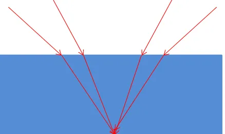
In two or multimedia photogrammetry refraction is the key issue to deal with. The refraction according to Snell’s Law reduces the opening angle of a camera when viewing from air into water due to the higher refractive index of water. As one can see from Figure 1, the refraction may also lead to a smaller ray intersection angle in 3D coordinate determination from stereo imagery and thus degrade the depth coordinate precision when imaging through the optical media air- water, Maas, 2015, figure 1.
Figure 1: Reduced forward intersection angle in two-media photogrammetry
Additionally, the variation of the refractive index over the visible part of the electro-magnetic spectrum is 1.4% in water, while it is only 0.008% in air, Maas, 2015. Shorter wavelength light experiences a stronger refraction than longer wavelength light, leading to color seams (red towards the nadir point, blue outward) in RGB images. The blurriness will reduce the image quality as well as the image measurement precision potential.
The experimental base for this contribution are several test flights along and off the coast with varying water depth (< 3.5 m) and sea floor conditions. In a preliminary test flight it became clear, that common commercial software products such as Agisoft Photoscan and Pix4DMapper will not be able to derive reliable key points and subsequently no exterior orientation in a mixed land / water block from images with are 100 % over water. Therefore two scenarios were developed. The first along a promenade pier with water depth of up to 3.5 m and the second one along a beach with groynes and in a distance of 50 to 60 m and water depth of approx. 2.5 m.
Sunny and cloud free weather is normally stated as a prerequisite for airborne and satellite remote sensing. But in an
aquatic environment the sun may also cause problems, such as sun glitter and glare. These two effects can be minimized by flying in the morning hours and under conditions with no of only little waves. UAS remote sensing allow us to operate below the clouds, thus it is possible to avoid the problems of sun glitter and glare. Therefore, one test flight was also conducted at overcast skies to investigate the differences due to varying weather conditions.
During photogrammetric processing of UAS imagery using SFM algorithm automatic key point matching requires static surfaces and linear line of sight between the sensor and the object, which is not the case in our scenario. Nevertheless, it is of importance to see how different software products are able to deal with this special data.
At deeper waters the completeness the accuracy and the proportion of noise of the derived dense point cloud will be subject of the investigations. Due to the air/water transition and different refraction of water and air the off nadir angle is important for the accuracy of the matching. With high image overlap the resection angles can maybe limited in order to enhance the accuracy of the final results. Due to expected mismatches a thorough filtering and noise removal of the point cloud is necessary. Figure 2 describes the general workflow of the paper in the left column and the specific investigations and research on the right column.
Figure 2: Developed general workflow for coastal under water DEM (left column) and conducted research for calibration and quality assessment (right column)
Automatic key
point detection
Filter of under
water points
Integrated sensor
orientation
UAS Aerial Survey
Dense Point cloud
generation
Noise reduction /
Filter / smoothing
Refraction
Correction
Coastal under
water DEM
Software
Comparison
Test of different
strategies
Software
Comparison
Quality
Assessment
Quality
Assessment
Manual vs.
automatic
Weather / viewing
angle
2 TEST FLIGHTS HEILIGENDAMM
As a test site for practical experiments a promenade pier in the coastal village Heiligendamm of an approximate length of 150m was chosen. A total of three test flights (9th, 14th and 17th of March) with different environmental conditions were conducted. Along the pier and on the beach 12 GCP's were collected with a RTK-GPS receiver. The approximate accuracy of the GCP's is 1-2 cm horizontally and 2-3 cm vertically. The flights were planned with an endlap and sidelap of 80 / 80 %. The flights were conducted with a Falcon 8 trinity UAS from Ascending Technologies. The camera mounted on the UAS is a Sony Alpha 7R with 36 Mpix. and a 35 mm fixed lens. The chosen GSD of 1 cm resulted in a flight height of approx. 70 m and a total of 88 images. Due to a malfunction of the barometric sensor the actual flight height of the test flights was between 84 - 87 m a.s.l. Thus the practical endlap was even more than the anticipated 80 %. The test site was covered with 4 flight strips along the promenade pier. The water depth around the pier reaches a maximum of approx. 3.5 m.
Additionally to the UAS flight over the promenade pier two flights along the shore were performed (14th and 17th of March). At that section of the shore groynes form protective structures of tropical wood and extend from the shore into the water to prevent the beach from washing away. The length of the groynes into the water is approximately 40 m. The water depth at the tip of the groynes is between 2 - 2.5 m. The test site was also covered with 4 flight strips along the shore. The flight parameters GSD and overlap are similar to the one over the pier. In order to test the influence of the incidence angle against the water and also extending the covered area on the ground, the second flight on March 17th was performed turning the camera approx. 20° off nadir, thus using an oblique perspective. In order to minimize blur the shutter speed was set to 1/800 s for all flights. Compensation for the different amount of light was given by different f-stop values, ranging from 2.8 - 5.6.
The first test flight was conducted at 9th of March 2016 from 11:44 - 11:48 under sunny conditions. The water was quite clear and the sea bottom clearly visible. Due to the mainly southeasterly wind, blowing off shore, only small waves were visible. The second flight test flight was conducted at 14th of March 2016 from 11:10 - 11:14 and 11:22 – 11:27 under overcast conditions. The water was relatively clear and the sea bottom visible. Due to the westerly wind, blowing along the shore significant waves of 10 - 25 cm were observed. Unknown reasons lead to two missing images of the groynes flight, which subsequently caused the geotagging software of the UAS to crash, thus no initial geolocations could be generated for this flight. The third flight was carried out three days later at 17th of March 2016 from 09:24 - 09:28 again under sunny conditions. The water was very clear and the sea bottom visible. The gentle westerly wind, blowing along the shore small generated waves of 2 - 5 cm. The relevant environmental conditions of all three flights are summarized in the following table 1.
Weather data comes from the weather station on the promenade pier itself. Information about the water level etc. is used from the Station Warnemünde, approx. 20 km away, provided by the state network of Mecklenburg-Vorpommern. Sun position was calculated with the freeware Tool LunaSolcalc. Salinity information was derived from the Prediction Model Salinity of the Federal Maritime and Hydrographic Agency BSH.
Table1: Environmental conditions during UAS test flights
Description Flight 1 Flight 2 Flight 3 Date 09.03.2016 14.03.2016 17.03.2016
Time 11:44 -
2.1 Importance of flight weather conditions
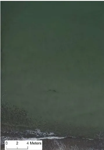
Using UAS imagery with a very high spatial resolution even the small waves generate a significant light pattern at sunny weather conditions, see figure 3 of the first flight. The net like wave pattern is more visible over sandy and shallow grounds. At deeper waters and over darker ground the light pattern becomes less visible. These patterns, which of course change their positions between neighboring images causes significant problems during image point matching, thus resulting in noise, especially in shallow waters, as a detailed view of the same spot in two consecutive images demonstrates, figure 4.
Figure 4: "Moving" wave patterns between neighbouring images of flight 1 under sunny conditions
At overcast weather conditions the disturbing light patterns disappear and the wave pattern is not visible in the images anymore, see figure 5 from the second flight. The waves also cause a white water zone directly at the shore line, thus making it impossible for image matching in this zone.
Figure 5: Flight 2 under overcast flight conditions - no visible wave pattern
2.2 Photogrammetric data processing
The five data sets of the three different dates have been processed with Agisoft Professional (Vers. 1.23). Additionally, the first data set has been processed with Pix4D Photomapper (Vers. 2.0) in order to investigate if there are significant differences in the data processing and the results between common commercial software products. According to the general photogrammetric workflow, in a first step the images are automatically oriented using Structure-From-Motion (SFM) algorithm and SIFT and SURF like operators for the identification of key points. The SFM method uses a number of images that generally depict a static area or a single object from several arbitrary viewpoints and attempts to recover the interior and exterior orientation parameters and a sparse point cloud that represents the 3D geometry of that scene. Bundle adjustment methods are used to improve the accuracy of calculating the camera trajectory and to minimize the projection error. Waves introduce a “moving” water column and generate spatially varying patterns on the see floor, as seen from figure 3 and 4,
thus introducing difficulties in the matching process. As the key requirement of static features for key point identification in the images is only valid for the non-water portions of the images, the distribution of the key points for further bundle adjustment and integrated sensor orientation is restricted to the pier, the groynes and the beach. Key points over water bodies can be considered as mismatches and should be removed.
Due to the uneven distribution of key points and ground control points (GCP’s) the results of the integrated sensor orientation for the pier flights are far from perfect. The determined EO parameters differ significantly (several meters) between the two commercial software products Photoscan and Pix4Dmapper in position and height, figure 6.
Figure 6: Estimated exterior orientation derived with two different software packages of image block "Pier" Flight 1, 09.03.2016. Background image digital orthophoto (State Survey Mecklenburg-Vorpommern)
It is clearly visible from figure 6 that Pix4Dmapper has had serious problems with the alignment. But that does not necessarily imply that the determined EO-parameters with Photoscan are correct. The residuals at the ground control points, however are minimal (2 – 3 cm RMS) for both software products. From this experience Photoscan was chosen as the software product for further processing.
The calculated radial distortion of the different test flights is quite similar, except for the second pier flight. The reason for it is unclear, but it is most probably related to the fact of the missing initial GPS values, figure 7.
Tab. 1: Calculated focal length of nadir flights over the promenade pier
Flight 1 Flight 2 Flight 3 Focal length 36.8415 36.9385 37.0692
xcp 0.1449 0.128 0.1504
ycp 0.0731 0.1103 0.2243
Tab. 2: Calculated focal length of off nadir flights over the beach and the groynes
Flight 1 Flight 2 Focal length 36.114 36.1452
xcp 0.1713 0.1668 ycp 0.0517 0.0178
Figure 7: Radial distortion profiles of Sony Alpha 7R, derived from the five test flights
With respect to completeness and noise the dense point clouds generated by Photoscan professional (vers. 1.23) differed significantly between the three different flights, figure 8 thus showing the significant influence of the environmental circumstances of the UAS flights.
Figure 8: Dense point clouds of the test site "pier". Computed with Photoscan, flight 1,2,3, from left to right.
Best results for dense point cloud generation with Photoscan were achieved by generating a “low” point density cloud using an “aggressive” depth filtering. The "low" point density option means an a priori downscaling (smoothing) of the images to a
1/16th of the original image. For the dense point cloud computation Photoscan normally uses a pair wise SGM-like method for image-matching, if you use the "Height-field, exact or smooth option". Only the "Fast" method utilizes a multi-view approach, Agisoft, 2016. The reasons for the noise are related to the unknown quality of the exterior orientation, but also to the water and wave induced movements and the two media photogrammetry related problems.
The software SURE from N-Frames (Wenzel et al., 2013) was used to investigate the influencing factors for image matching using SGM for photo bathymetry in more detail. From the theory and the results of the commercial software products tested it became apparent, that there might be two screws to improve the number of the correctly determined points. Firstly, a small forward intersection angle to minimize the refraction problem, but with the drawback of imprecise height determination accuracy. Secondly, a pair wise stereo matching and not using multiple images for matching, thus reducing the possibilities of mismatches, but with the drawback of potential noise. The results reveal that the SURE point clouds, computed with the above mentioned parameters are more complete but also much noisier than the point clouds from photoscan, see figure 9 and 10 for the example of the groynes flight 1.
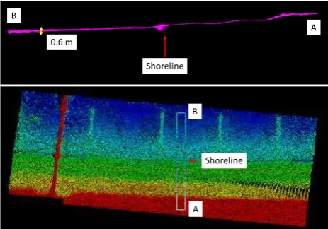
Figure 9: Dense point cloud and cross section of first flight groynes, computed with Photoscan
Figure 10: Dense point cloud and cross section of first flight groynes, computed with SURE
The post processing of the raw points clouds is done in a batch routine, including several steps with the software LAStools
-60.0 -40.0 -20.0 0.0 20.0 40.0 60.0 80.0 100.0 120.0 140.0
1 2 3 4 5 6 7 8 9 10 11 12 13 14 15 16 17 18 19 20 21
D
isto
rti
o
n
[µ
m]
Radial Distance [mm] Pier I Pier II Pier III Groynes I Groynes II
4
0 -3 Height
0.6 m
Shoreline
Shoreline
A B
A B
3 m
Shoreline
Shoreline
A B
from Rapidlasso GmbH. In a preprocessing step the initial point clouds from Photoscan or SURE are compressed into the LAZ-format to speed up further processing (las2las). In a first filtering step all points above the water level and points below -4 m are removed (las2las). In a second filtering step the remaining noise below the bottom line has to be identified and removed (lascanopy). Therefore the 20 percent tiles are computed and the identified points below become removed. The third step classifies the remaining point cloud into ground and non-ground points (lasheight, lasground). Thereby non ground points are located at the remains of the pier and the groynes. Finally, the grounds points are interpolated to a grid of 2 m cell size.
The depth accuracy of the collected data is a very important question in our investigation. The UAS photogrammetric data are compared against reference data from the sea bottom. The reference data is not only important for validation but also for the determination of the refraction correction factor. In a first surveying campaign the shallow waters of up to 1 m below sea level were surveyed with a RTK GPS by foot. The second more systematic survey was conducted with a small boat on April 5th. A total station on the beach measured the reflector on top of a 4 m pole. The boat allowed also to measure the sea bottom at water depth of up to 3.4 m. The vertical accuracy of the terrestrial measurements is 3 - 4 cm, because of the ripple structure of the sandy sea bottom and the antenna pole which sometimes sinks a little into the ground. The total of 255 measured observations with an approximate distance of 30 m were interpolated into a reference DTM with a grid size of 1 m using geostatistical methods (kriging). Due to the gentle profile of the sandy beach the average prediction error of the interpolated DTM is only between 3 - 5 cm. See figure 10 for the reference DTM.
Figure 11: Reference Data - Digital Depth Model based on terrestrial and boat survey, Background image digital orthophoto (State Survey Mecklenburg-Vorpommern)
2.3 Refraction correction
The refractive index of water depends on the optical wavelength as well as water temperature, salinity and depth and can be obtained from an empirical formula as used in HÖHLE, 1971:
��= 1.338 + 4∗10−5(486− �+ 0.003�+ 50� − �)
(with nw = refractive index of water, d = water depth (m), λ =
wave length (nm), T = water temperature (°C), S = water salinity (%)).
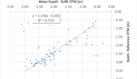
In our case the refraction index varies between 1.348 and 1.352. Bagheri et al., 2015, did not use the theoretical refractive index, but calculated an empirical one. The empirical refraction coefficient was derived thru a regression analysis of the filtered point cloud against the measured reference data. Regressions were computed for the different flights and the tests with the point cloud software products. A selected number are presented in figures 12 – 16. The graphs reveal the differences between the flights, the varying success of the filtering and the differences between the two test sites.
Figure 12: Pier Flight t 1 – Filtered point cloud SURE vs. -3.50 -3.00 -2.50 -2.00 -1.50 -1.00 -0.50 0.00
D
Water Depth - SURE DTM [m]
y = 0.892x - 0.100 -4.00 -3.00 -2.00 -1.00 0.00
D
Water Depth - Agisoft DTM [m]
y = 1.068x - 0.100 -4.00 -3.00 -2.00 -1.00 0.00
D
Figure 15: Groynes Flight 1 - Filtered point cloud SURE vs. reference DTM
Figure 16: Groynes Flight 1 - Filtered point cloud Photoscan vs. reference DTM
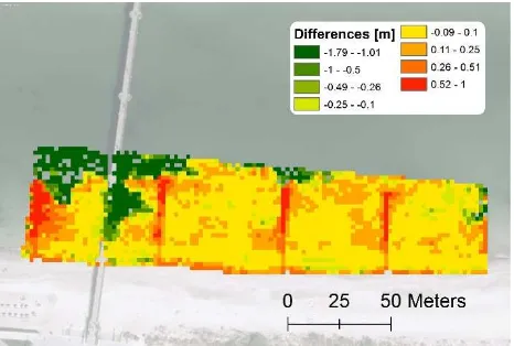
3 ACCURACY ASSESSMENT
The differences between the refraction corrected photogrammetric bathymetric DTM and the reference bathymetric DTM are shown in fig. 17 and fig. 18. They reveal that UAS photogrammetry is capable to deliver reasonable results if all the preprocessing steps are done with great care, but may also be subject to large errors.
Figure 17: Differences between bathymetric reference DTM
and refraction corrected DTM of the 2nd flight “pier”,
computed with SURE
Figure 18: Differences between bathymetric reference DTM
and refraction corrected DTM of the 1st flight “groynes”,
computed with Photoscan
For the 1st groynes flight with overcast skies, the majority (50.7 %) of the grid cells exhibits only a small difference of ± 0.1 m. A further 25.7 % of the points are observed at a difference from ± 0.1 m to ± 0.25 m. Only 11 % show strong deviations of more than 1 m. In particular, in the shallow regions (for example in the eastern part of the test site), the differences are very small.
4 CONCLUSIONS AND OUTLOOK
From a practitioner’s perspective one has to conclude, that it is feasible to determine the shallow sea bottom from a UAS survey with a certain degree of accuracy. However, there are limitations and pitfalls. The key to a reliable under water DTM are most suitable weather conditions, which are: overcast sky and no or little waves during the UAS aerial survey. The images should be taken from a nadir perspective, because an oblique view will cause additional problems due to the increasingly reduced forward intersection angle in two-media photogrammetry. Secondly careful data processing and filtering of the data. For initial relative orientation enough above ground features have to be visible in the image block. "Pure" water images cannot be integrated in the block, due to two reasons: the prerequisite of stable image patterns for key point determination and the refraction of the water. Image blocks fully over water will produce a different set of interior orientation parameters, taking the refraction into account, e.g. Agrafiotis & Georgopoulos, 2015, Telem, & Filin, 2010. Different software products will deliver different results. The quality of the dense point cloud is related to the accuracy of the integrated sensor orientation, the internal filter algorithms and the post processing procedure. Refraction correction is necessary. The application of the theoretical refraction correction factor is applicable, if the whole data processing chain is able to eliminate the noise and gross errors.
In general, the present study demonstrates that the photo bathymetric DTM acquired by UAS photogrammetry give promising results, but there is more research necessary to fully investigate the potential of the proposed approach. Further research will also focus on better point cloud generation and filtering and the comparison of photo bathymetry vs. opto empirical bathymetry.
5 REFERENCES
Agisoft (2016): Agisoft community forum - Topic: Algorithms used in Photoscan (= http://www.agisoft.com/forum/index.php? topic=89.msg323#msg323
Water Depth - SURE DTM [m]
y = 1.344x - 0.100
Agrafiotis, P. and Georgopoulos, A. (2015): Camera Constant in the case of two Media Photogrammetry.- Int. Arch.
Photogramm. Remote Sens. Spatial Inf. Sci., Volume XL-5/W5,
2015 Underwater 3D Recording and Modeling, 16–17 April 2015, Piano di Sorrento, Italy
Bagheri, O.; Ghodsian, M.; Saadatseresht, M. (2015): Reach scale application of UAV+SFM method in shallow rivers hyperspatial bathymetry.- IAPRS, Vol. XL-1/W5, 2015 - International Conference on Sensors & Models in Remote Sensing & Photogrammetry, 23–25 Nov 2015, Kish Island, Iran
Costa, B. M.; Battista, T. A. & Pittman, S. J. (2009): Comparative evaluation of airborne LiDAR and ship-based multibeam SoNAR bathymetry and intensity for mapping coral reef ecosystems. Remote Sensing of Environment, 113(5), p. 1082-1100.
Flener, C.; Lotsari, E.; Alho, P. & Käyhkö, J. (2012): Comparison of empirical and theoretical remote sensing based bathymetry models in river environments. River Research and Applications 2012, 28:1, 118-133.
Guenther, G. C., Cunningham, A. G., Laroque, P. E., Reid, D. J. (2000): Meeting the accuracy challenge in airborne Lidar bathymetry. Proceedings of the 20th EARSeL Symposium: Workshop on Lidar Remote Sensing of Land and Sea, Dresden, Germany, 28p.
Höhle, J. (1971): Zur Theorie und Praxis der Unterwasser-Photogrammetrie. In Schriften der DGK; Verlag der Bayerischen Akademie der Wissenschaften: München, Germany; Vol. 163.
Javernick, L.; Brasington, J.; Caruso, B. (2014): Modeling the topography of shallow braided rivers using Structure-from-Motion photogrammetry, Geomorphology, Vol. 213: 166-182.
LunaSolCalc
(=http://www.vvse.com/products/de/lunasolcal.html) accessed, 9.03.2016
Maas, H.-G. (2015): On the Accuracy Potential in Underwater/Multimedia Photogrammetry.- Sensors 2015, 15, 18140-18152; doi:10.3390/s150818140
Mancini, A.; Frontoni; E. Zingaretti, P.; Longhi. S. (2015): High-resolution mapping of river and estuary areas by using unmanned aerial and surface platforms.- 2015 International Conference on Unmanned Aircraft Systems (ICUAS) Denver, Colorado, USA, June 9-12, 2015, p. 534 - 542
Needham, H. & Hartmann, K. (2013): Imagery-derived Bathymetry and Seabed Classification Validated. Hydro
International, Vol. 17. p. 14 - 17
Niemeyer, J.; Kogut, T. & Heipke, C. (2014): Airborne Laser Bathymetry for Monitoring the German Baltic Sea Coast.
Tagungsband der DGPF-Jahrestagung, 10 p.
Prediction Model Salinity - Geowebservice (https://www.geoseaportal.de/wss/service/PredictionModel_Wat erSalinity/guest) accessed, 9.03.2016
Jordt-Sedlazeck, A. & Koch, R. (2013): Refractive Structure-from-Motion on Underwater Images.- Computer Vision
(ICCV), 2013 IEEE International Conference on, 2013, pp 57-64.
Telem, G.; Filin, S. (2010): Photogrammetric modeling of underwater environments.- ISPRS J. Photogramm. Remote
Sens., Vol. 65, pp. 433–444.
Murase, T.; Tanaka, M.; Tani, T.; Miyashita, Y.; Ohkawa, N.; Ishiguro, S.; Suzuki, Y.; Kayanne, H.; Yamano, H. (2008): A Photogrammetric Correction Procedure for Light Refraction Effects at a Two-Medium Boundary.- PE&RS, Vol. 74, No. 9, September 2008, pp. 1129–1136
Westaway, R.M.; Lane, S.N.; and Hicks, D.M. (2001): Remote Sensing of Clear-Water, Shallow, Gravel-Bed Rivers Using Digital Photogrammetry.- PE&RS, Vol. 67, No. 11, pp. 1271-1281.
Wenzel, K., Rothermel, M.; Haala, N. (2013): SURE – The ifp Software for Dense Image Matching.- In: Fritsch, D. [Ed.]:
Photogrammetric Week 2013.- pp. 59 - 70. Wichmann Verlag.
Williams, R. D., Brasington, J., Vericat, D. and Hicks, D. M. (2014), Hyperscale terrain modelling of braided rivers: fusing mobile terrestrial laser scanning and optical bathymetric mapping. Earth Surf. Process. Landforms, 39: 167–183.
Woodget, A., et al. (2015). "Quantifying submerged fluvial topography using hyperspatial resolution UAS imagery and structure from motion photogrammetry." Earth Surface