Time-Series analysis of MODIS NDVI data along with ancillary data for Land use/Land
cover mapping of Uttarakhand
KEY WORDS: Land use/land cover, NDVI, MODIS, Phenology, MOD13Q1.
ABSTRACT:
Land use and land cover plays an important role in biogeochemical cycles, global climate and seasonal changes. Mapping land use and land cover at various spatial and temporal scales is thus required. Reliable and up to date land use/land cover data is of prime importance for Uttarakhand, which houses twelve national parks and wildlife sanctuaries and also has a vast potential in tourism sector. The research is aimed at mapping the land use/land cover for Uttarakhand state of India using Moderate Resolution Imaging Spectroradiometer (MODIS) data for the year 2010. The study also incorporated smoothening of time-series plots using filtering techniques, which helped in identifying phenological characteristics of various land cover types. Multi temporal Normalized Difference Vegetation Index (NDVI) data for the year 2010 was used for mapping the Land use/land cover at 250m coarse resolution. A total of 23 images covering a single year were layer stacked and 150 clusters were generated using unsupervised classification (ISODATA) on the yearly composite. To identify different types of land cover classes, the temporal pattern (or) phenological information observed from the MODIS (MOD13Q1) NDVI, elevation data from Shuttle Radar Topography Mission (SRTM), MODIS water mask (MOD44W), Nighttime Lights Time Series data from Defense Meteorological Satellite Program (DMSP) and Indian Remote Sensing (IRS) Advanced Wide Field Sensor (AWiFS) data were used. Final map product is generated by adopting hybrid classification approach, which resulted in detailed and accurate land use and land cover map.
1. INTRODUCTION
Land Use and Land Cover (LULC) play a vital role in understanding the complex earth’s ecosystem processes, biogeochemical cycles (Achard et al., 2004; Liu et al., 2008; Sellers et al., 1997), climate change studies (Liu et al., 2004) and deforestation studies(Hansen et al., 2008; Skole and Tucker, 1993; Steininger et al., 2002). Land use and land cover information is extensively used by various governmental and non-governmental organizations and thus placing a great demand on detailed, reliable and up to date LULC maps (Perera and Tsuchiya, 2009). International Geosphere Biosphere Program (IGBP 1990), Intergovernmental Panel on Climate Change (IPCC 1990), National Research Council (NRC 2005), and Global Terrestrial Observation systems (GTOS 2009) etc., have identified land use and land cover as an important driver for climate change. Land use/land cover also impacts the socio-economic conditions of the people (Hietel et al., 2005; Lo and Yang, 2002; Ribeiro and Lovett, 2009; Swetnam et al., 2011) and hence detailed scientific study is required in this field for better environmental planning, management and conservation.
Before the era of satellite remote sensing, mapping of land resources started with manual interpretation of aerial photographs (Colwell, 1960). These techniques were tedious and time consuming. Global land cover data sets were first prepared using various published maps, atlases, national sources and ground level surveys (Matthews, 1983; Olson et al., 1983). The global land cover maps generated by this method suffered lack of consistency in classification schema used, differences in spatial resolutions and variables in measurement techniques(Running et al., 1994; Townshend et al., 1991).
Land use land cover mapping of larger areas using satellite remote sensing started with National Oceanic and Atmospheric Administration (NOAA) Advanced Very High Resolution Radiometer (AVHRR) data. (Nemani and Running, 1997).
Various Global land cover data sets were prepared using multi temporal AVHRR NDVI data sets (De Fries et al., 1998; IGBP DISCover, Loveland et al., 2000; UMD GLCC, Hansen et al., 2000). Major disadvantages of using AVHRR data is its poor geometric accuracy and limited radiometric calibration (Cihlar et al., 1997; Meyer et al., 1995).
Global Land Cover (GLC) 2000 maps were produced making use of SPOT VEGETATION data (Agrawal et al., 2003; Bartholomé and Belward, 2005; Han, 2004; Mayaux et al., 2006; Stibig et al., 2007). NDVI data derived from VGT sensor is also utilized for national level mapping of vegetation cover (Vancutsem et al., 2009; Xiao et al., 2002).
Land use land cover mapping is also possible using multi resolution data obtained from various satellite platforms like Landsat (Bakr et al., 2010; Huang et al., 2009; Olthof and Fraser, 2007; Steininger et al., 2002), Indian Remote Sensing IRS-1C satellite based Wide Field Sensor (WiFS) data with 189 meter resolution (Joshi et al., 2001, 2006) and Indian Remote Sensing IRS-P6 satellite based Advanced Wide Field Sensor (AWiFS) data with 56 meter resolution (Kandrika and Roy, 2008). However, these data sets suffer limitations in terms of spatial coverage, temporal resolution and availability of cloud free data (Asner, 2001; Hansen et al., 2008; Song et al., 2001).
Several researchers demonstrated the use of MODIS vegetation Indices to produce land use land cover maps (Clark et al., 2010; García-Mora et al., 2012; Klein et al., 2012; Thenkabail et al., 2005; Wardlow et al., 2007; Zhang et al., 2008). In the present study, MOD13Q1 vegetation indices product at 250m resolution was used.
Present study has the advantage of (i) Using temporal plots of various land cover classes to understand the status of the vegetation, (ii) Smoothening the time-series curves to eliminate the erroneous interpretations, (iii) Use of ancillary data to Sandeep Kumar Patakamuria*, Shefali Agrawalb, and M. Krishnavenia
a Centre for Water Resources, Anna University, Guindy, Chennai, India-600 025 b Indian Institute of Remote Sensing, 4-Kalidas Road, Dehradun, India-248001
support classification decision making and (iv) Use of land use land cover maps derived from AWiFS data alongside with high resolution Google earth imagery as reference data for classification accuracy assessment. The approach presented in this study is expected to have better accuracy and is adoptable for land use land cover mapping at different geographical locations.
2. STUDY AREA AND DATA DESCRIPTION Uttarakhand is a state located in the northern region of India with a geographical extent of 53,483 km2. The state is situated
between 28o 43' to 31o 27' N latitudes and 77o 34' to 81o 02' E
longitudes (Figure. 1). It is bordered by the Tibet autonomous region on the north, Nepal on the east and the Indian states of Uttar Pradesh to the south, Haryana to the west and Himachal Pradesh to the North West. Climate of the state falls into temperate zone and tropical zone with temperatures varying from sub-zero to 43o C. Elevation values ranges from 200 m to
8000m above mean sea level and supports a variety of flora and fauna (Forest Survey of India, 2011; Ministry of Economics and Statistics, 2010). Topography and climate plays a major role in ecology, socio economic status and culture of the people in this region (SoE, 2004). Agriculture is the major sector in this area and many industries are forest dependent. There are over fifteen important rivers and over a dozen glaciers in the state. Uttarakhand has over two hundred medium to large sized hydro-projects and these projects highly influence the environment and living conditions of the people (Rana et al., 2007; WSMD, 2009).
The state is housing six national parks, six wild life sanctuaries and two conservation reserves. The state is one of the major contributors of the tourism sector in India, attracting several domestic and international tourists. The state also has a rich and ancient cultural heritage and is also called as Dev-Bhoomi which means land of Gods. Uttarakhand state is sensitive to natural calamities like flash floods; landslides and earth quakes and requires well planned environmental management system. In September 2010 Uttarakhand has faced floods due to heavy rain fall resulting in loss of lives and property (Sharma, 2012).This study can help planners and decision makers to better manage and protect the land resources of Uttarakhand.
In the present study, MODIS 250m resolution vegetation indices product MOD13Q1 is used for mapping the land use land cover of Uttarakhand. The product contains 16-day composite of Normalized Difference Vegetation Index (NDVI), Enhanced Vegetation Index (EVI), blue, red, near infrared (NIR), mid-infrared (MIR) and pixel reliability (Huete et al., 2002, 1999; Solano et al., 2010). Entire study area is covered by two MODIS tiles numbered H24V05 and H24V06. “Data required for the present study was obtained through the online Data Pool at the NASA Land Processes Distributed Active Archive Center (LP DAAC), USGS/Earth Resources Observation and Science (EROS) Center, Sioux Falls, South Dakota (https://lpdaac.usgs.gov/get_data)" with the help of United States Geological Survey (USGS) Earth Explorer (EE) tool (http://earthexplorer.usgs.gov/).
Ancillary data collected for the study includes Digital Elevation Model (DEM) data derived from Shuttle Radar Topographic Mission (SRTM) (Farr et al., 2007; Jarvis et al., 2008) downloaded from Consortium for Spatial Information website
(
http://www.cgiar-csi.org/data/srtm-90m-digital-elevation-database-v4-1#download). MODIS land water mask
(MOD44W) product derived from MODIS and SRTM data (Carroll et al., 2009) downloaded from LP DAAC, Defense Meteorological Satellite Program (DMSP) Operational Linescan System (OLS) nighttime lights time series data downloaded from National Geophysical Data Center
(http://ngdc.noaa.gov/eog/dmsp/downloadV4composites.html),
Advanced Wide Field Sensor (AWiFS) imagery downloaded from Bhuvan portal developed by National Remote Sensing Centre Open Earth Observation Data Archive (NOEDA) to visualize and disseminate earth observation data (
http://bhuvan-noeda.nrsc.gov.in/download/download/download.php), and
Land use land cover maps at 1:250,000 scale derived using AWiFS, obtained from National Remote Sensing Centre, Department of Space, Government of India, Hyderabad.
Figure 1. Location map of the study area- Uttarakhand
3. METHODS
The methods adopted in this study can be broadly divided into five stages: (i) Data preparation, (ii) Image classification, (iii) Generating time-series plots and smoothening, (iv) Grouping the classes based on similarity and (v) Accuracy assessment. The flow chart depicted in Figure. 2 represents the systematic approach adopted in the present study.
3.1 Data Preparation
A total of 23 tiles for H24V05 and 23 tiles of H24V06 covering the study area were downloaded for the year 2010 starting from January to December. These images were then mosaicked together to form 23 images, and later layer stacked to form annual composite image.
3.2 Image classification
1996; Richards and Jia, 1999). MODIS data was grouped to 150 clusters with 25 iterations and a convergence threshold of 0.95. The classification resulted in 105 useful clusters with non-zero values.
3.3 Generating time-series plots and smoothening Once the classification process was finished, a set of four random samples were collected from each of the 105 clusters and multi-temporal NDVI plots were generated for each of the 420 sample locations.
There are several factors such as atmospheric conditions, sensor viewing geometry, cloud cover, aerosol concentrations, off-nadir viewing and low sun zenith angles that causes noise in NDVI time series (Gutman, 1991; Holben and Fraser, 1984; Kobayashi and Dye, 2005; Li and Strahler, 1992). Savitzky-Golay filtering technique was used in this study to filter the noise in NDVI response. It is a simplified least squares fit convolution for smoothing and computing derivatives of a spectrum (Savitzky and Golay, 1964).
3.4 Grouping the classes based on similarity
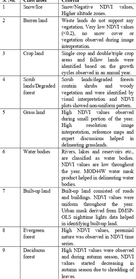
The clusters with similar temporal characteristics were grouped together based on the theory that similar land cover classes exhibit similar temporal patterns. Time-series patterns of sample points were extracted from each cluster, elevation data, image interpretation of AWiFS false color composites and Google earth visual interpretation helped in proper identification of land use/land cover classes. Table.1 below shows the criteria followed in attributing suitable land use/land cover class to each cluster.
3.5 Accuracy assessment
Accuracy assessment is a key stage in thematic mapping using remotely sensed data. Classification accuracy assessment indicates the qualitative aspects of the land cover map. It determines whether the generated map serves the purpose of the users or not. Accuracy assessment is a complex process involving several problems of consideration (Foody, 2008, 2002).
In this study, accuracy assessment is carried out using error matrix. It accounts for commission errors, as well as omission errors and kappa statistics which reflects the difference between actual agreement and the agreement expected by chance (Lillesand and Kiefer, 2008).
Reference data for accuracy assessment is collected with the help of National land use and land cover maps derived by using multi-temporal AWiFS for the year 2009-2010 and Google Earth (GE) image interpretation. Stratified random sampling is used with a minimum of 25 samples per class, and a total of 300 sample points were generated. Grids were generated with 250 x 250 m size for each of the sample point to match the pixel size of the MODIS NDVI data and exported to Google Earth for visualization.
S. No. Class label Criteria
1 Snow/Ice Snow/Negative NDVI values, Higher altitude zones.
2 Barren land Waste lands do not support any vegetation. Very low NDVI values (<0.2), no snow cover or vegetation observed during image interpretation.
3 Crop land Single crop and double/triple crop areas and fallow lands were identified based on the growth cycles observed in an annual year.
4 Scrub
lands/Degraded forest
Scrub lands/degraded forests contain shrubs and woody vegetation and were identified by visual interpretation and NDVI plots showed non-uniform pattern. 5 Grass land High NDVI values observed
during small portion of the year. High resolution image interpretation, reference maps and expert discussions helped in delineating grasslands.
6 Water bodies Rivers, lakes and reservoirs etc., are classified as water bodies. uniform throughout the year. Urban mask derived from DMSP-OLS nighttime lights data helped in identifying built-up land. 8 Evergreen
forest High NDVI values, perennial nature was observed in NDVI time series.
9 Deciduous
forest High NDVI values were observedand during autumn season, NDVI values started decreasing in autumn season due to shredding of leaves.
Table 1. Criteria followed in identification and attribution of land use/ land cover class names to each cluster
4. RESULTS AND DISCUSSIONS 4.1 Plotting NDVI time-series and smoothening
(a)
(b)
(c)
(d)
(e)
(f)
(g)
(h)
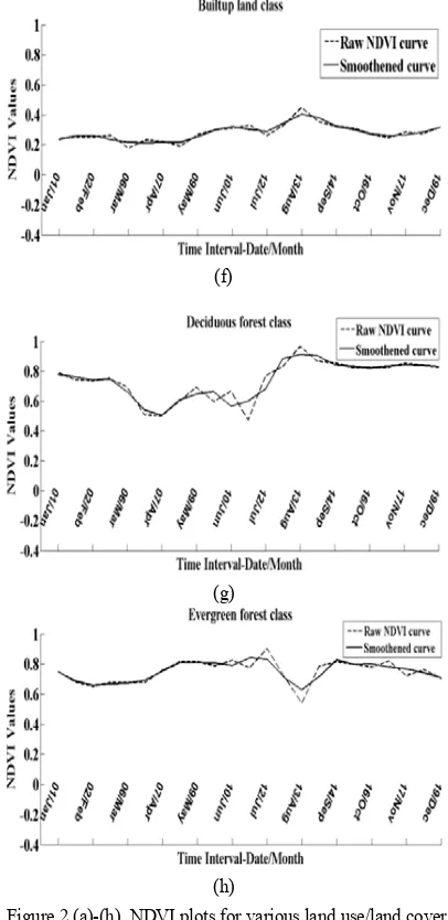
Figure 2 (a)-(h). NDVI plots for various land use/land cover classes namely (a).Snow/Ice, (b).Barren land, (c).Grass land, (d).Shrub land/Degraded forest, (e).Crop land, (f).Built-up
land, (g).Deciduous forest, and (h). Evergreen forest, and their smoothened response to Savitzky-Golay filer.
(Figure. 2 (e)). Built-up lands consist of buildings, roads and a small portion of urban vegetation. NDVI values are of lower amplitude (<0.4) and plots followed fairly uniform pattern (Figure. 2 (f)). Decreasing pattern of the NDVI plots in the deciduous class is associated with shredding of leaves during autumn season (Figure. 2 (g)). Evergreen forests showed high NDVI values throughout the year and minute amplitude disturbances are in response to the canopy moisture content during wet seasons (Figure. 2 (h)).
4.2 Ancillary reference collection
Present study made use of several ancillary reference datasets like SRTM DEM, MODIS Water mask, DMSP-OLS nighttime lights time series data, AWiFS imagery and Google Earth© high resolution imagery. All these data sets were re-projected to the spatial resolution of MODIS imagery. SRTM DEM data was used to identify elevation values which helped in differentiating land cover classes. Water mask and nighttime lights data helped in classification of water bodies and built-up lands respectively.
For collecting Google earth reference data, rectangular grids were generated with side length of 250 meters around each of the 420 sample points that were collected during time-series plots generation. Various land cover classes of the present study were viewed in Google earth as shown in Figure. 3.
(a)
(b)
(c)
(d)
(e)
(f)
(g)
(h)
Figure 3 (a)-(h). Various land use/land cover classes as visualized in Google Earth (a).Snow/Ice, (b).Barren lands, (c).Grass lands, (d).Shrub lands/Degraded forest, (e).Crop lands, (f).Built-up land, (g).Deciduous forest, (h).Evergreen
forest.
Reference grids were created to match the spatial resolution of MODIS pixels. Many researchers have used google earth imagery for classification and validation of land use/land cover maps (Clark et al., 2010; Colditz et al., 2012). When a mixed class is observed inside the grid, the majority land cover type (>70%) present in the grid is allocated for the sample. Snow/Ice class was observed at higher altitudes and fresh snow appeared brighter than permanent snow. Barren lands support minimum to no vegetation cover and these samples were easily differentiated from other classes based on texture information. Shrub lands/degraded forest is a land cover class consisting of trees and shrubs. Crop lands were identified by rectilinear shapes and plow lines and slope agriculture was identified with the help of elevation information. Identification of grass lands was a difficult task experienced in the study. Grass lands were mixed with crop lands and shrub land classes, and differentiating these classes was found to be a challenging task. Built-up lands contained man made buildings and road networks. Evergreen forests were differentiated from deciduous frosts with the help of elevation information. Deciduous forests are located at the lower altitude zones compared to evergreen forests as deciduous forest could not adapt to the cold and dry weather at high altitudes. No shedding of leaves was observed in evergreen forests during autumn season.
4.3 Final Classification and map compilation
All the clusters belonging to a particular land use/land cover class were recoded at the final stage of classification Urban mask derived from DMSP-OLS Night time lights data and water mask derived from MOD44W product were appended to the final land use/land cover map of Uttarakhand for the year 2010. Map generated in the present study is presented on a reduced scale in Figure. 4.
Figure 4.Land use/land cover map of Uttarakhand for the year 2010 on a reduced scale
4.4 Evaluation of mapping results
Results obtained in the present study were evaluated in both qualitative and quantitative aspects. Reference map classes were aggregated to match the classification schema of the present study for quantitative validation. Area statistics for all the classes were calculated for the present map and compared with the area extent of reference map obtained from Bhuvan portal (Aggarwal et al., 2012) as shown in Table. 2. Results were also compared with Forest Survey of India publication (FSI) statistics published in India State of Forest report 2011.
Land use/land
Table 2. Area statistics of land use/land cover map derived in the present study compared with reference map
It is observed that the results obtained are in close agreement with the area statistics of the reference data. Minor over estimation in water bodies and built-up lands are attributed to the use of urban mask and water mask in delineating these land cover classes. Differences in the remaining land cover classes may be attributed to the moderate resolution of the imagery used in the study. According to Forest Survey of India report, the total forest area in Uttarakhand is 24,766 sq.km and non-forest area is 28,717 sq. km (Forest Survey of India, 2011). When aggregated, the present study results showed a total forest area of 26,563 sq. km and non-forest area of 26,920 sq. km.
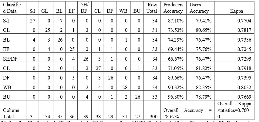
Qualitative aspects of the thematic mapping effort were validated using error matrix (Lillesand and Kiefer, 2008) generated with the help of three hundred sample points obtained by stratified random sampling method. NRSC-ISRO land use/land cover map for the year 2009-2010 was used as reference image for the purpose of validation. Rectangular reference grids were generated for all three hundred points with dimensions of 250m x 250m for the purpose of visualization on Google Earth. Spatial distortions occurred in the google earth reference will be negligible compared to the pixel size of the imagery used in the study (Clark et al., 2010). Table. 3 represent the error matrix, producers accuracy, users accuracy and kappa statistics of the accuracy assessment process.
Error matrix obtained in the present study clearly highlights the complex nature of accuracy assessment. Present study incorporated careful examination of sample locations on multiple source like published reference maps, google earth as well as AWiFS imagery for assuring the quality of classification. The result showed an overall accuracy of 78.67% with over all kappa statistics of 0.7600.
5. CONCLUSION
During the land use and land cover mapping of Uttarakhand, barren lands, dry river beds, fallow lands and portions of the built-up land exhibited similar temporal pattern at some of the locations. In order to better delineate Built-up lands and Water bodies, the study made use of urban mask derived from DMSP-OLS nighttime lights time series data and water mask derived from MOD44W product. Identification of grass lands and shrub lands/mixed forest classes is observed to be a difficult task as the temporal patterns were difficult to interpret and differentiate in these classes. It is thereby suggested to consider for more number of sample locations at these clusters. Elevation information obtained from SRTM DEM data helped in differentiating various vegetation classes. Prior knowledge about the study area and suitable reference datasets also plays a major role in improving the quality of classification. It is of prime importance to have a clear definition and classification criteria for each land use/land cover type used in a particular mapping exercise.
Time series plots generated in the study may contain disturbances due to sensor geometry, atmospheric errors and sensor calibrations. Savitzky-Golay filtering was adopted in the present study to smoothen the time-series curves and there by avoid erroneous interpretations. The study incorporated the visual interpretation of google earth imagery in classification and accuracy assessment phases. With recent advancement in web based GIS it would be a great opportunity to deploy crowd sourcing in which experts from the field, research collaborators and volunteers can collectively work at various stages of land cover classification and validation.
Land use/land cover map generated in the present study was evaluated in both qualitative and quantitative aspects. Over all accuracy of the present map is found to be 78.67% with over all kappa coefficient of 0.7600. The methods and techniques used in the study demonstrated the ability of multi-temporal NDVI data in mapping land use/land cover. Various governmental, non-governmental and research organizations can make use of
the results (available
athttp://doi.pangaea.de/10.1594/PANGAEA.816654) obtained
Classifie
d Data S/I GL BL EF SH/ DF CL DF WB BU TotalRow ProducersAccuracy UsersAccuracy Kappa
S/I 27 0 7 0 0 0 0 0 0 34 87.10% 79.41% 0.7704
GL 0 25 2 1 3 0 0 0 0 31 73.53% 80.65% 0.7817
BL 4 3 26 0 0 0 0 1 0 34 74.29% 76.47% 0.7336
EF 0 4 0 25 2 1 1 0 0 33 69.44% 75.76% 0.7245
SH/DF 0 0 0 4 26 3 1 0 0 34 66.67% 76.47% 0.7295
CL 0 2 0 1 2 27 0 0 1 33 71.05% 81.82% 0.7918
DF 0 0 0 5 0 3 26 0 0 34 89.66% 76.47% 0.7395
WB 0 0 0 0 2 4 0 28 0 34 90.32% 82.35% 0.8032
BU 0 0 0 0 4 0 1 2 26 33 96.30% 78.79% 0.7669
Column
Total 31 34 35 36 39 38 29 31 27 300 Overall Accuracy = 78.67%
Overall Kappa statistics=0.760 0
S/I: Snow/Ice, GL: Grass lands, BL: Barren lands, EF: Evergreen forest, SH/DF: Shrub/degraded forest, CL: crop lands, DF: Deciduous forest, WB: Water bodies and BU: Built-up lands.
Table 3. Error matrix for the land use/land cover map of Uttarakhand
ACKNOWLEDGEMENTS
The authors would like to thank Indian Institute of Remote Sensing, Dehradun and Anna University, Chennai for providing an opportunity to carry out this work. MODIS data products were obtained at the NASA Land Processes Distributed Active Archive Center (LPDAAC), USGS/EROS center. National land use/land cover map was obtained from National Remote Sensing Centre/ISRO.
REFERENCES
Achard, F., Eva, H.D., Mayaux, P., Stibig, H.-J., Belward, A., 2004. Improved estimates of net carbon emissions from land cover change in the tropics for the 1990s. Global Biogeochem. Cycles 18, 1–11. doi:10.1029/2003GB002142
Aggarwal, S., Shadab, S., Karnatak, H.C., 2012. Thematic Data Dissemination on Bhuvan Gateway to Indian Earth
Observation, in: Open Source Geospatial Resources to Spearhead Development and Growth. pp. 1–5.
Agrawal, S., Joshi, P.K., Shukla, Y., Roy, P.S., 2003. SPOT VEGETATION multi temporal data for classifying vegetation in south central Asia. Mater. Chem. 84, 157–163.
Asner, G.P., 2001. Cloud cover in Landsat observations of the Brazilian Amazon. Int. J. Appl. Earth Obs. Geoinf. 22, 3855– 3862.
Bakr, N., Weindorf, D.C., Bahnassy, M.H., Marei, S.M., El-Badawi, M.M., 2010. Monitoring land cover changes in a newly reclaimed area of Egypt using multi-temporal Landsat data. Appl. Geogr. 30, 592–605.
doi:10.1016/j.apgeog.2009.10.008
Bartholomé, E., Belward, a. S., 2005. GLC2000: a new approach to global land cover mapping from Earth observation data. Int. J. Remote Sens. 26, 1959–1977.
doi:10.1080/01431160412331291297
Carroll, M.L., Townshend, J.R., DiMiceli, C.M., Noojipady, P., Sohlberg, R. a., 2009. A new global raster water mask at 250 m resolution. Int. J. Digit. Earth 2, 291–308.
doi:10.1080/17538940902951401
Chen, J., Jönsson, P., Tamura, M., Gu, Z., Matsushita, B., Eklundh, L., 2004. A simple method for reconstructing a high-quality NDVI time-series data set based on the Savitzky–Golay filter. Remote Sens. Environ. 91, 332–344.
doi:10.1016/j.rse.2004.03.014
Chen, X., Mithal, V., Vangala, S.R., Brugere, I., Boriah, S., Kumar, V., 2011. A study of time series noise reduction techniques in the context of land cover change detection. Dep. Comput. Sci. Eng. Reports 11–016.
Cihlar, J., Ly, H., Li, Z., Pokrant, H., 1997. Multitemporal , Multichannel AVHRR Data Sets for Land Biosphere Studies Artifacts and Corrections. Remote Sens. Environ. 60, 35–57. doi:10.1016/S0034-4257(96)00137-X
Clark, M.L., Aide, T.M., Grau, H.R., Riner, G., 2010. A scalable approach to mapping annual land cover at 250 m using MODIS time series data: A case study in the Dry Chaco ecoregion of South America. Remote Sens. Environ. 114, 2816–2832. doi:10.1016/j.rse.2010.07.001
Colditz, R.R., López Saldaña, G., Maeda, P., Espinoza, J.A., Tovar, C.M., Hernández, A.V., Benítez, C.Z., Cruz López, I., Ressl, R., 2012. Generation and analysis of the 2005 land cover map for Mexico using 250m MODIS data. Remote Sens. Environ. 123, 541–552. doi:10.1016/j.rse.2012.04.021
Colwell, R.N., 1960. Manual of photographic interpretation. The American society of photogrammetry.
Dwyer, M., Schmidt, G., 2006. The MODIS reprojection tool. Earth Sci. Satell. Remote Sens. 162–177.
Farr, T., Rosen, P., Caro, E., 2007. The shuttle radar topography mission. Rev. Geophys. 15, 1–33. doi:10.1029/2005RG000183.1.INTRODUCTION
Foody, G.M., 2002. Status of land cover classification accuracy assessment. Remote Sens. Environ. 80, 185–201.
doi:10.1016/S0034-4257(01)00295-4
Foody, G.M., 2008. Harshness in image classification accuracy assessment. Int. J. Remote Sens. 29, 3137–3158.
doi:10.1080/01431160701442120
Forest Survey of India, 2011. India State of Forest Report 2011, in: India State of Forest Report 2011. Forest Survey of India, Dehradun, pp. 236–240.
doi:http://www.fsi.org.in/cover_2011/uttarakhand.pdf
Fritz, S., McCallum, I., Schill, C., Perger, C., See, L., Schepaschenko, D., van der Velde, M., Kraxner, F., Obersteiner, M., 2012. Geo-Wiki: An online platform for improving global land cover. Environ. Model. Softw. 31, 110– 123. doi:10.1016/j.envsoft.2011.11.015
García-Mora, T.J., Mas, J.-F., Hinkley, E.A., 2012. Land cover mapping applications with MODIS: a literature review. Int. J. Digit. Earth 5, 63–87. doi:10.1080/17538947.2011.565080
Gutman, G., 1991. Vegetation indices from AVHRR: An update and future prospects. Remote Sens. Environ. 35, 121– 136.
Han, K., 2004. A land cover classification product over France at 1 km resolution using SPOT4/VEGETATION data. Remote Sens. Environ. 92, 52–66. doi:10.1016/j.rse.2004.05.005
Hansen, M.C., Defries, R.S., Townshend, J.R.G., Sohlberg, R., 2000. Global land cover classification at 1 km spatial resolution using a classification tree approach. Int. J. Remote Sens. 21, 1331–1364. doi:10.1080/014311600210209
Hansen, M.C., Stehman, S. V, Potapov, P. V, Loveland, T.R., Townshend, J.R.G., DeFries, R.S., Pittman, K.W., Arunarwati, B., Stolle, F., Steininger, M.K., Carroll, M., DiMiceli, C., 2008. Humid tropical forest clearing from 2000 to 2005 quantified by using multitemporal and multiresolution remotely sensed data. Proc. Natl. Acad. Sci. U. S. A. 105, 9439–9444.
Herold, M., Mayaux, P., Woodcock, C.E., Baccini, a., Schmullius, C., 2008. Some challenges in global land cover mapping: An assessment of agreement and accuracy in existing 1 km datasets. Remote Sens. Environ. 112, 2538–2556. doi:10.1016/j.rse.2007.11.013
Hietel, E., Waldhardt, R., Otte, A., 2005. Linking socio-economic factors, environment and land cover in the German Highlands, 1945–1999. J. Environ. Manage. 75, 133–143. doi:10.1016/j.jenvman.2004.11.022
Hird, J.N., McDermid, G.J., 2009. Noise reduction of NDVI time series: An empirical comparison of selected techniques. Remote Sens. Environ. 113, 248–258.
doi:10.1016/j.rse.2008.09.003
Holben, B., Fraser, R., 1984. Red and near-infrared sensor response to off-nadiir viewing. Int. J. Remote Sens. 5, 145–160. doi:10.1080/01431168408948795
Huang, C., Kim, S., Song, K., Townshend, J.R.G., Davis, P., Altstatt, A., Rodas, O., Yanosky, A., Clay, R., Tucker, C.J., Musinsky, J., 2009. Assessment of Paraguay’s forest cover change using Landsat observations. Glob. Planet. Change 67, 1–12. doi:10.1016/j.gloplacha.2008.12.009
Huete, a, Didan, K., Miura, T., Rodriguez, E.., Gao, X., Ferreira, L.., 2002. Overview of the radiometric and biophysical performance of the MODIS vegetation indices. Remote Sens. Environ. 83, 195–213. doi:10.1016/S0034-4257(02)00096-2
Huete, A., Justice, C., Leeuwen, W. Van, 1999. MODIS Vegetation index alogrithm theoritical basis document, Algorithm theoretical basis ….
Jarvis, A., Reuter, H.I., Nelson, A., Guevara, E., 2008. Hole-filled SRTM for the globe, Version 4. CGIAR-CSI SRTM 90m Database. Int. Cent. Trop. Agric. Cali, Columbia. http//srtm. csi. cgiar. org.
Jensen, J.R., 1996. Introductory digital image processing. Prentice Hall New Jersey, New Jersey.
Jones, K.B., Survey, U.S.G., Discipline, B., 2006. Importance of Land Cover and Biophysical Data in Landscape-Based Environmental Assessments, in: North America Land Cover Summit. pp. 215–250.
Jonsson, P., Eklundh, L., 2002. Seasonality extraction by function fitting to time-series of satellite sensor data. Geosci. Remote Sens. 40, 1824–1832.
Joshi, P.K., Singh, S., Agarwal, S., 2001. Land cover assessment in Jammu & Kashmir using phenology as discriminant – An approach of wide swath satellite ( IRS – WiFS ). Curr. Sci. 81, 392–399.
Joshi, P.K.K., Roy, P.S., Singh, S., Agrawal, S., Yadav, D., 2006. Vegetation cover mapping in India using multi-temporal IRS Wide Field Sensor (WiFS) data. Remote Sens. Environ. 103, 190–202. doi:10.1016/j.rse.2006.04.010
Justice, C.O., Townshend, J.R.G., Holben, B.N., Tucker, C.J., 1985. Analysis of the phenology of global vegetation using meteorological satellite data. Int. J. Remote Sens. 6, 1271– 1318. doi:10.1080/01431168508948281
Kandrika, S., Roy, P.S., 2008. Land use land cover
classification of Orissa using multi-temporal IRS-P6 awifs data: A decision tree approach. Int. J. Appl. Earth Obs. Geoinf. 10, 186–193. doi:10.1016/j.jag.2007.10.003
Klein, I., Gessner, U., Kuenzer, C., 2012. Regional land cover mapping and change detection in Central Asia using MODIS time-series. Appl. Geogr. 35, 219–234.
doi:10.1016/j.apgeog.2012.06.016
Li, X., Strahler, A., 1992. Geometric-optical bidirectional reflectance modeling of the discrete crown vegetation canopy: Effect of crown shape and mutual shadowing. IEEE Trans. Geo Sci. Remote Sens. 30, 276–292.
Lillesand, T.M., Kiefer, R.W., 2008. Remote sensing and image interpretation, Distribution. Wiley.
Liu, J., Liu, S., Loveland, T.R., Tieszen, L.L., 2008. Integrating remotely sensed land cover observations and a biogeochemical model for estimating forest ecosystem carbon dynamics. Ecol. Modell. 219, 361–372. doi:10.1016/j.ecolmodel.2008.04.019
Liu, S., Kairé, M., Wood, E., Diallo, O., Tieszen, L.L., 2004. Impacts of land use and climate change on carbon dynamics in south-central Senegal. J. Arid Environ. 59, 583–604. doi:10.1016/j.jaridenv.2004.03.023
Lo, C.P., Yang, X., 2002. Driver of Land-Use/Cover Changes and Dynamic Modeling for the Atlanta, Georgia Metropolitan Area. Photogramm. Eng. Remote Sensing 68, 1073–1082.
Lu, D., Weng, Q., 2007. A survey of image classification methods and techniques for improving classification performance. Int. J. Remote Sens. 28, 823–870. doi:10.1080/01431160600746456
Matthews, E., 1983. Global vegetation and land use: New high-resolution data bases for climate studies. J. Clim. Appl. Meteorol. 22, 474–487.
Mayaux, P., Eva, H., Gallego, J., Strahler, A.H., Herold, M., Agrawal, S., Naumov, S., Miranda, E.E. De, Bella, C.M. Di, Ordoyne, C., Kopin, Y., Roy, P.S., 2006. Validation of the global land cover 2000 map. IEEE Trans. Geosci. Remote Sens. 44, 1728–1739. doi:10.1109/TGRS.2006.864370
Meyer, D., Verstraete, M., Pinty, B., 1995. The effect of surface anisotropy and viewing geometry on the estimation of NDVI from AVHRR. Remote Sens. Rev. 12, 3–27.
doi:10.1080/02757259509532272
Ministry of Economics and Statistics, 2010. Uttarakhand at a Glance 2010-11. Dehradun.
Morisette, J.T., Privette, J.L., Justice, C.O., 2002. A framework for the validation of MODIS Land products. Remote Sens. Environ. 83, 77–96. doi:10.1016/S0034-4257(02)00088-3
Nemani, R., Running, S., 1997. Land cover characterization using multitemporal red, near-IR, and thermal-IR data from NOAA/AVHRR. Ecol. Appl. 7, 79–90. doi:10.1890/1051-0761(1997)007[0079:LCCUMR]2.0.CO;2
Olson, J.S., Watts, J.A., Allison, L.J., 1983. Carbon in live vegetation of major world ecosystems. ORNL.
Olthof, I., Fraser, R., 2007. Mapping northern land cover fractions using Landsat ETM+. Remote Sens. Environ. 107, 496–509. doi:10.1016/j.rse.2006.10.009
Perera, K., Tsuchiya, K., 2009. Experiment for mapping land cover and it’s change in southeastern Sri Lanka utilizing 250m resolution MODIS imageries. Adv. Sp. Res. 43, 1349–1355. doi:10.1016/j.asr.2008.12.016
Rana, N., Sati, S.P., Sundriyal, Y.P., Doval, M., Juyal, N., 2007. Socio-economic and environmental implications of the hydroelectric projects in Uttarakhand Himalaya, India. J. Mt. Sci. 4, 344–353. doi:10.1007/s11629-007-0344-5
Ribeiro, S.C., Lovett, A., 2009. Associations between forest characteristics and socio-economic development: a case study from Portugal. J. Environ. Manage. 90, 2873–81.
doi:10.1016/j.jenvman.2008.02.014
Richards, J. a., Jia, X., 1999. Remote Sensing Digital Image Analysis. Springer Berlin Heidelberg, Berlin, Heidelberg. doi:10.1007/978-3-662-03978-6
Rouse, J., Haas, R., Schell, J., Deering, D., 1973. Monitoring vegetation systems in the Great Plains with ERTS., in: Third ERTS Symposium, Vol. 1. pp. 309–317.
Running, S.W., Loveland, T.R., Pierce, L.L., 1994. A Vegetation Classification Logic-Based on Remote-Sensing for Use in Global Biogeochemical Models. Ambio 23, 77–81.
Savitzky, A., Golay, M.J.E., 1964. Smoothing and Differentiation of Data by Simplified Least Squares Procedures. Anal. Chem. 36, 1627–1639. doi:10.1021/ac60214a047
Sellers, P.J., Dickinson, R.E., Randall, D.A., Betts, A.K., Hall, F.G., Berry, J.A., Collatz, G.J., Denning, A.S., Mooney, H.A., Nobre, C.A., Sato, N., Field, C.B., Henderson-Sellers, A., 1997. Modeling the Exchanges of Energy, Water, and Carbon Between Continents and the Atmosphere. Science (80-. ). 275, 502–209.
Sharma, S., 2012. Catastrophic hydrological event of 18 and 19 September 2010 in Uttarakhand, Indian Central Himalaya—an analysis of rainfall and slope failure. Curr. Sci. 102, 327–332.
Skole, D., Tucker, C., 1993. Tropical deforestation and habitat fragmentation in the Amazon: satellite data from 1978 to 1988. Science 260, 1905–10. doi:10.1126/science.260.5116.1905
SoE, U., 2004. Uttaranchal Status of Environment, in: Environment Protection and Pollution Control board,Uttarakhand.
Solano, R., Didan, K., Jacobson, A., Huete, A., 2010. MODIS Vegetation Index User ’ s Guide ( MOD13 Series ).
Song, C., Woodcock, C.E., Seto, K.C., Lenney, M.P., Macomber, S.A., 2001. Classification and Change Detection Using Landsat TM Data When and How to Correct Atmospheric Effects? Remote Sens. Environ. 75, 230–244. doi:10.1016/S0034-4257(00)00169-3
Steininger, M.K., Tucker, C.J., Townshend, J.R.G., Killeen, T.J., Desch, A., Bell, V., Ersts, P., 2002. Tropical deforestation in the Bolivian Amazon. Environ. Conserv. 28, 127–134. doi:10.1017/S0376892901000133
Swetnam, R.D., Fisher, B., Mbilinyi, B.P., Munishi, P.K.T., Willcock, S., Ricketts, T., Mwakalila, S., Balmford, A., Burgess, N.D., Marshall, A.R., Lewis, S.L., 2011. Mapping socio-economic scenarios of land cover change : A GIS method to enable ecosystem service modelling. J. Environ. Manage. 92, 563–574. doi:10.1016/j.jenvman.2010.09.007
Thenkabail, P.S., Schull, M., Turral, H., 2005. Ganges and Indus river basin land use/land cover (LULC) and irrigated area mapping using continuous streams of MODIS data. Remote Sens. Environ. 95, 317–341. doi:10.1016/j.rse.2004.12.018
Townshend, J., Justice, C., Li, W., Gurney, C., McManus, J., 1991. Global land cover classification by remote sensing: present capabilities and future possibilities. Remote Sens. Environ. 35, 243–255. doi:10.1016/0034-4257(91)90016-Y
Vancutsem, C., Pekel, J.-F., Evrard, C., Malaisse, F., Defourny, P., 2009. Mapping and characterizing the vegetation types of the Democratic Republic of Congo using SPOT
VEGETATION time series. Int. J. Appl. Earth Obs. Geoinf. 11, 62–76. doi:10.1016/j.jag.2008.08.001
Wardlow, B., Egbert, S., Kastens, J., 2007. Analysis of time-series MODIS 250 m vegetation index data for crop classification in the U.S. Central Great Plains. Remote Sens. Environ. 108, 290–310. doi:10.1016/j.rse.2006.11.021
White, M. a., 2005. A global framework for monitoring phenological responses to climate change. Geophys. Res. Lett. 32, L04705. doi:10.1029/2004GL021961
WSMD, 2009. Uttarakhand State Perspective and Strategic Plan. Watershed Management Directorate, Dehradun, pp. 105– 108.
Xiao, X., Boles, S., Liu, J., Zhuang, D., Liu, M., 2002. Characterization of forest types in Northeastern China, using multi-temporal SPOT-4 VEGETATION sensor data. Remote Sens. Environ. 82, 335–348.
doi:10.1016/S0034-4257(02)00051-2