LABORATORY FLUME EXPERIMENT WITH A CODED STRUCTURED LIGHT
SYSTEM
Devrim Akca a, *, and Hansjorg Seybold b a
Dept. of Civil Engineering, Isik University, 34980 Sile, Istanbul, Turkey
bDept. of Earth, Atmospheric, and Planetary Sciences, MIT, Cambridge, MA 02139-4307 USA –
Commission V, WG V/6
KEY WORDS: Geomorphology, geophysics, monitoring, DEM/DTM, multitemporal, river deltas.
ABSTRACT:
The topography of inland deltas is influenced chiefly by the water‐sediment balance in distributary channels and local evaporation and seepage rates. In a previous study, a reduced complexity model has been applied to simulate the process of inland delta formation. Results have been compared with the Okavango Delta, Botswana and with a laboratory experiment. Both in the macro scale and the micro scale cases, high quality digital elevation models (DEM) are essential. This work elaborates the laboratory experiment where an artificial inland delta is generated on laboratory scale and its topography is measured using a Breuckmann 3D scanner. The space-time evolution of the inland delta is monitored in the consecutive DEM layers. Regarding the 1.0m x 1.0m x 0.3m size of the working area, better than 100 micron precision is achieved which gives a relative precision of 1/10 000. The entire 3D modelling workflow is presented in terms of scanning, co-registration, surface generation, editing, and visualization steps. The co-registered high resolution topographic data allows us to analyse the stratigraphy patterns of the experiment and gain quantitative insight into the spatio-temporal evolution of the delta formation process.
* Corresponding author.
1. INTRODUCTION
Inland deltas can be found in several places around the world, e.g. in Botswana (Okavango), the Sudan (The Sudd) or Slovakia (Danube). Although the plan view of diverging channel networks looks quite similar, inland deltas and coastal deltas are morphologically very distinct. Inland deltas are dominated by channel flow influenced by evapotranspiration, infiltration, and the growth of bank and island‐stabilizing vegetation. Because of these additional complex processes and feedbacks, inland deltas are less well studied than their coastal counterparts.
For describing the long-term dynamics of the sediment transport and the evolution of the delta on geological scale, new models have to be developed, reducing the complexity of the hydrological and sedimentary equation but still keeping the essential physics (Paola and Leeder, 2011). Results have to be compared with field data and laboratory-scale experiments requiring high quality digital elevation models (DEM). Recently, Seybold et al. (2010) have developed such a model, so called reduced complexity model to study the formation of inland deltas, with application to the Okavango Delta. A former version of the model simulates the formation of coastal deltas (Seybold et al., 2007, 2009). This model has been extended to include water loss to describe the morphogenesis of inland deltas.
The work has been accompanied by a laboratory-scale flume experiment where the morphology of the different sedimentation patterns has been analyzed in spatial and temporal domains (Seybold et al., 2010).
This paper focuses on the measurement and analysis aspects of the flume experiment. A micro scale artificial inland delta is generated in laboratory conditions. The formation process lasts two days. The surface topography is measured with a high accuracy Breuckmann 3D scanner at five data epochs. Each epoch is represented in a separate DEM layer.
The Breuckmann 3D scanner is based on a coded structured light method, in which regular fringes are projected onto the surface and the stripes’ deformations are measured using a CCD camera. From the deformations of these stripes the topography can be reconstructed with an accuracy of 100 microns (Akca, 2012).
The technical details of the laboratory set-up and the 3D scanner are given in the next chapter. The third chapter presents the 3D modelling workflow from data acquisition to high quality DEM generation. The geomorphologic analyses are given in the fourth chapter.
1.1 Close Range Morphological Measurement for the Earth Sciences
The laboratory flume experiments on delta formation have been carried out in the last years by several laboratories (Hoyal and Sheets, 2009; Martin et al., 2009). Also, the formation of alluvial fans caused by rapid water release has been studied by Kraal et al. (2008).
These papers emphasize on the study of the geomorphologic patterns, while the geodetic and photogrammetric works in terms of surface measurement and DEM generation have not been discussed in detail.
The close range morphological measurement for the Earth sciences is an active research area in photogrammetry since long time. The analytical and digital photogrammetric methods have been used for the precise measurement of land surface topography, surface roughness and river bank dynamics (Kirby, 1991; Pyle et al., 1997; Merel and Farres, 1998). In the recent years, laser scanning systems have also been used for rapid and dense point cloud data acquisition tasks (Milan et al., 2007; Hodge et al., 2009).
2. FLUME EXPERIMENT
2.1 Laboratory Set-up
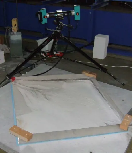
The flume setup consists of a 1 x 1 meter aluminium basin, which is fixed at an inclination of about 6 degrees. The main slope runs along the diagonal of the basin. An initial surface is created using a uniformly sloped sediment layer with a height of 5 centimetres at the inlet (Figure 1a and 1b).
(a)
(b)
Figure 1. The test setup.
We use crushed glass as sediment with diameter 50 to 120 microns and a bulk density of ρ = 2.2 g/cm3. The sediment is continuously mixed with water using a marine-type impeller in an upstream tank. This mixture is injected at a steady rate into the basin using a peristaltic pump. The volumetric sediment concentration is approximately 0.05 and the inflow is set to 1000 ml/h. To simulate the boundary conditions of the dry delta, infiltrated water which accumulates at the bottom edge is continuously pumped out. In addition water is evaporated by an array of fifteen 300W heat lamps that are fixed 15 cm above the surface.
The experiment is run as follows: a water/sediment mixture is injected into the flume over 45 minutes, followed by drying over 2:15 hours. We call one period of injection and drying an
“epoch”, where epoch 0 denotes the initial condition (Figure 1b). After complete drying of each epoch, the surface topography is scanned using a Breuckmann OptoTOP‐SE 3D scanner. Data for five epochs have been collected: epochs 0, 1, 2, 3 and 4 where epoch 0 denotes the initial surface. The complete drying is necessary to avoid specular reflections produced by the wet sand; these reflections would otherwise disturb the scanning.
2.2 Breuckmann OptoTOP-SE 3D scanner
The optoTOP-SE system (Figure 2), as a high definition topometrical 3D-scanner, allows the 3-dimensional digitization of objects with high resolution and accuracy. The optoTOP-SE system uses special projection patterns with a combined Gray code and phase shift technique, which guarantees an unambiguous determination of the recorded 3D data with highest accuracy (Breuckmann, 2003).
Figure 2. Breuckmann optoTOP-SE scanner.
Table 1. Technical specifications of the optoTOP-SE sensor.
Field of View (mm) 400 x 315
Depth of View (mm) 260
Acquisition time (sec) < 1.0
Weight (kg) 2 – 3
Digitization (points) 1280 x 1024
Base length (mm) 300
Triangulation angle (deg) 30
Projector pattern 128 order sinus
Lamp 100W halogen
Lateral resolution (micron) ~300 Feature accuracy (relative) 1/10000 Feature accuracy (micron) ~50
The time for a single scan takes about 1 second for a 1.4 mega pixel camera. The sensor of the optoTOP-SE system can be scaled for a wide range of Field of Views (FOV), by changing International Archives of the Photogrammetry, Remote Sensing and Spatial Information Sciences, Volume XXXIX-B5, 2012
the baseline distance and/or lenses, typically between a few centimetres up to several meters. Thus, the specifications of the sensor can be adapted to the special demands of a given measuring task. The factory specifications of the system are given in Table 1.
3. 3D MODELLING
The 3D modelling workflow comprises of the scanning, co-registration, surface generation, editing, and visualization steps.
3.1 Scanning
The Breuckmann optoTOP-SE is a very light and flexible scanning system. It can easily be oriented towards the object of interest using a stable tripod. Since the system has only 40.0 x 31.5 cm FOV in the best scanner-to-object viewing angle, several scans have to be performed in order to cover the entire object. Thus, planning the scan overlay needs careful preparation.
In each epoch, 13–15 point clouds (Table 2) have been scanned in order to cover the entire flume area. Each point cloud consists of 1’280 x 1’204 = 1’310’720 points with their X, Y, Z and intensity values. The average point spacing is 35 microns in all data sets.
The scanning step of a single epoch took 1-2 hours of working time. The whole project lasted in two days.
3.2 Co-registration and surface generation
Due to the limited FOV of the scanner, several scans have to be performed. These scans (in the form of point clouds) are combined into a co‐registered mosaic to cover the entire surface of the related epoch, using the least square 3D surface matching (LS3D) method (Gruen and Akca, 2005; Akca, 2010).
The LS3D method is a rigorous algorithm for the matching of overlapping 3D surfaces and point clouds. It estimates the transformation parameters of one or more fully 3D surfaces with respect to a template surface, using the generalised Gauss– Markov model, minimising the sum of the squares of the Euclidean distances between the surfaces. This formulation gives the opportunity to match arbitrarily oriented 3D surfaces, without using explicit tie points.
In the LS3D approach, when more than two pint clouds with multiple overlaps exist, as in the case of this experiment, a two step solution is adopted. In the first step, the pairwise LS3D matchings are performed on every overlapping pair and a subset of point correspondences is saved to separate files. In the consequent global registration step, all these files are passed to a block adjustment by the independent models procedure, in which all residual errors are evenly distributed among all the point clouds. Details of the procedure can be found in Akca (2010).
For example, epoch0 in Table 2 contains 14 point clouds, which results in 18.4 million points in total. The 14 point clouds have 24 overlapping pairs. The average of the standard deviations of these 24 pairwise LS3D computations is 68.3 microns. The final global registration step concludes with a standard deviation value of 42.4 microns.
Table 2. Numerical results of the inner-epoch co-registration computations.
Once the point clouds of each epoch are co-registered, they are re-sampled into a DEM with using the SCOP++ version 5.4.2 International Archives of the Photogrammetry, Remote Sensing and Spatial Information Sciences, Volume XXXIX-B5, 2012
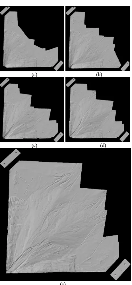
interpolation software. The point spacing is chosen as 300 microns. Thus, the spatial characteristic of the flume surface at each epoch is represented in an individual DEM layer (Figure 3).
At this point, the spatial characteristics of the 5 epochs are represented by the associated 5 DEMs whose coordinates are still not in a common system. In order to perform the spatio-temporal analysis, all DEMs have to be transformed into a common spatial coordinate system. We chose the epoch0 as the spatial datum, and co-register the remaining 4 DEMs with the reference frame of epoch0 using the LS3D algorithm. The numerical results are given in Table 3.
Since the flume surface has changed in the course of the experiment, only the stable surface parts (see ‘T’ signs at the upper left and lower right parts of Figure 3e) are considered in the computation.
Table 3. Numerical results of the cross-epoch co-registration computations.
By co‐registering the different sediment epochs, we obtain an insight into the spatial and temporal distribution of the sediment patterns. We apply 3D comparison techniques in order to quantitatively analyse the change in surface (Figure 4).
(a) (b)
(c) (d)
(e)
Figure 4. The spatial comparisons between the DEMs of epoch0−epoch1 (a), epoch0–epoch2 (b), epoch0–epoch3 (c), epoch0–epoch4 (d), and the residual bar in millimetres unit (e).
4. GEOMORPHOLOGICAL ANALYSIS
4.1 Slope Analysis
The morphology of the flume experiment can be analyzed by means of local elevation and topographic slope. The high resolution DEM is crucial to calculate the topographic slope accurately. Topographic slope can be used as a proxy for the dominant land forming processes. For example a decreasing slope is an indicator of a fluvial dominated surface evolution, while a constant or increasing slope indicates the dominance of hillslope processes.
To quantify the changes in the surface topography during the evolution of the delta experiment we calculate averaged slope <s> on rings of width dr = 5cm at different distances d from the inlet. The result is normalized by the overall mean slope of the system SM arriving at S(d) = <s>/SM.
The co-registered data allows us to analyze the changes of S(d) for each epoch. Clearly, three distinct regimes whose regions are marked in Figure 5 can be identified.
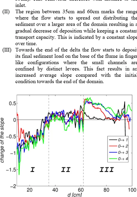
(I) A region where the sediment is transported in a well confined channel. Here, deposition increased with distance from the inlet resulting in a smaller average slope compared to the initial condition (distance 5cm-35cm). This behaviour decreases with distance to the inlet.
(II) The region between 35cm and 60cm marks the range where the flow starts to spread out distributing the sediment over a larger area of the domain resulting in a gradual decrease of deposition while keeping a constant transport capacity. This is indicated by a constant slope over time.
(III) Towards the end of the delta the flow starts to deposit its final sediment load on the base of the flume in finger like configurations where the small channels are confined by distinct levees. This fact results in an increased average slope compared with the initial condition towards the end of the domain.
Figure 5. Change in slope compared to the initial condition with distance from the inlet. The slope has been averaged over rings of width dr = 5cm for different distances d from the inlet and then normalized with the overall mean slope. Three regions
can be identified: I, II, and III.
4.1 Topography Dynamics
The different co-registered topographic layers can also be used to analyse the spatial evolution of the deposition pattern in time to gain insight into the stratigraphy of the delta formation process.
The total deposited volume of each epoch can be obtained by simply subtracting the DEM data from the previous one. For the four injections we obtain: V1 = 573 cm3, V2 = 904 cm3,
V3 = 614 cm3, V4 = 740 cm3, which gives an estimate of the variance of sediment input during the different runs.
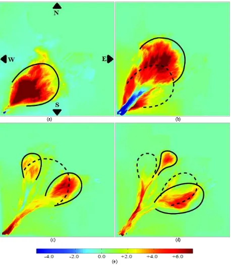
The spatial distribution of the sedimentation/erosion is illustrated in Figure 6, showing the change in surface elevation between successive epochs. Here, one can clearly identify the different deposition lobes for each epoch. The solid lines mark the boundaries of the current deposition zone and the dashed lines show the boundaries of the previous lobe.
(a) (b)
(c) (d)
(e)
Figure 6. Spatial distribution of the sedimentation and erosion between the successive epochs (a) epoch1–epoch0, (b) epoch2– epoch1, (c) epoch3–epoch2, (d) epoch4–epoch3. The residual bar is in millimetres unit (e).
During the first epoch the stream mainly deposits its sediment after a short inlet zone, filling up the domain and adjusting the initial slope to the transport capacity of the flow.
In the second injection the main flow direction is blocked by the first deposition lobe. Thus the stream first starts to incise a channel before it spreads out into a new fan on the left hand side of the former deposits (Figure 6b).
During the third deposition period the deposition inside the channel bed starts to occur forming a new sediment layer. The main deposition lobe switches to the east of the domain, while a new channel branch erodes through the side walls of the previous lobe forming a new lobe towards the north of the flume. In this and the following epochs, one can clearly see that initially sedimentation/erosion occurs only in a well confined channel until the stream spreads out and distributes its deposits in a larger domain forming the deltaic fan (Figure 6c and 6d).
5. CONCLUSIONS
In this work, the formation of inland deltas has been studied using a laboratory-scale flume experiment and DEM data analysis.
Novel high resolution scanning techniques have been applied, which allow us to measure detailed features of the experiment and analyze its surface morphology. The co-registered DEMs allow us to gain insight into the stratigraphy of the deposition pattern leading to a better understanding of the spatio-temporal dynamics of the delta formation process. Lobe switching and channel branching has been observed as in natural delta settings. The pattern formation mechanisms of the experiment and the resulting morphology are similar to those observed in nature, but on a different scale in space and time. The experimental results can serve as a tool to understand the interplay between the dominant sedimentation processes.
REFERENCES
Akca, D., 2010. Co-registration of surfaces by 3D Least Squares matching. Photogrammetric Engineering & Remote Sensing, 76 (3), 307-318.
Akca, D., 2012. 3D modeling of cultural heritage objects with a structured light system. Mediterranean Archaeology and Archaeometry, 12(1), to be appear.
Breuckmann B., 2003. State of the art of topometric 3D-metrology. In Proceedings of the Optical 3-D Measurement Techniques VI, Zurich, Switzerland, September 22-25, Vol. II, pp 152-158.
Gruen, A., and Akca, D., 2005. Least squares 3D surface and curve matching. ISPRS Journal of Photogrammetry and Remote Sensing, 59 (3), 151–174 .
Hodge, R., Brasington, J., and Richards, K., 2009. In situ characterization of grain-scale morphology using terrestrial laser scanning. Earth Surface Processes and Landforms, 34 (7), 954–968.
Hoyal, D., and Sheets, B., 2009. Morphodynamic evolution of cohesive experimental deltas. Journal of Geophysical Research, 114, F02009.
Kirby, R.P., 1991. Measurement of surface roughness in desert terrain by close range photogrammetry. Photogrammetric Record, 13 (78), 855 – 875.
Kraal, E., van Dijk, M., Postma, G., and Kleinhans M., 2008. Martian stepped‐delta formation by rapid water release. Nature, 451, 973–976.
Martin, J., Sheets, B., Paola, C., and Hoyal D., 2009. Influence of steady base‐level rise on channel mobility, shoreline migration, and scaling properties of cohesive experimental delta. Journal of Geophysical Research, 114, F03017.
Merel, A.P., and Farres, P.J., 1998. The monitoring of soil surface development using analytical photogrammetry. Photogrammetric Record, 16 (92), 331 – 345.
Milan, D.J., Heritage, G.L., and Hetherington, D., 2007. Application of a 3D laser scanner in the assessment of erosion and deposition volumes and channel change in a proglacial river. Earth Surface Processes and Landforms, 32 (11), 1657– 1674.
Paola, C., and Leeder, M., 2011, Environmental dynamics: Simplicity versus complexity. Nature, 469, 38-39.
Pyle, C.Y., Richards, K.S., and Chandler, J.H., 1997. Digital photogrammetric monitoring of river bank erosion. Photogrammetric Record, 15 (89), 753 – 764.
Seybold, H. J., Andrade Jr., J. S., and Herrmann, H. J., 2007. Modeling river delta formation. Proc. Natl. Acad. Sci. U. S. A., 104(43), 16 804–16 809, doi:10.1073/pnas.0705265104. Seybold, H. J., Molnar, P., Singer, H. M., Andrade Jr., J. S., Herrmann, H. J., and Kinzelbach, W., 2009. Simulation of birdfoot delta formation with application to the Mississippi Delta. Journal of Geophysical Research, 114, F03012.
Seybold, H.J., Molnar, P., Akca, D., Doumi, M., Cavalcanti Tavares, M., Shinbrot, T., Andrade Jr., J. S., Kinzelbach, W., and Herrmann H. J., 2010. Topography of inland deltas: Observations, modeling, and experiments. Geophysical Research Letters, 37 (8), L08402.