USING RELATIVE ORIENTATION CONSTRAINTS TO PRODUCE VIRTUAL IMAGES
FROM OBLIQUE FRAMES
A.M. G. Tommaselli a, M. V. A. Moraes a, J. Marcato Junior a , C. R. T. Caldeira a, R. F. Lopesb, M. Galoa
a Dept. of Cartography, Unesp - Univ Estadual Paulista, 19060-900 Pres. Prudente, SP, Brazil
{tomaseli, galo}@fct.unesp.br, {antunesdemoraes, jrmarcato}@gmail.com [email protected] b Aerocarta [email protected]
Commission I
KEY WORDS: Photogrammetry, Dual Head, camera calibration, fusion of multiple images.
ABSTRACT:
Image acquisition systems based on multi-head arrangement of digital cameras are attractive alternatives enabling larger imaging area when compared to a single frame camera. The calibration of this kind of systems can be performed using bundle adjustment with relative orientation stability constraints. The paper will address the details of the steps of the proposed approach for system calibration, image rectification, registration and fusion. Experiments with terrestrial and aerial images acquired with two Fuji FinePix S3Pro cameras were performed. The experiments focused on the assessment of the results of self calibrating bundle adjustment with and without relative orientation constraints and the effects in the registration and fusion when generating virtual images The experiments have shown that the images can be accurately rectified and registered with the proposed approach, achieving residuals smaller than 1 pixel.
1. INTRODUCTION
Digital medium format cameras have a favourable cost/benefit ratio when compared to high-end digital photogrammetric cameras and are also much more flexible to be used in different platforms and aircrafts. As a consequence, some companies are using professional medium format cameras in mapping projects, mainly in developing countries (Ruy et al, 2012). However, compared to large format digital cameras, medium format digital cameras have smaller ground coverage area, increasing the number of images, flight lines and also the flight costs.
One alternative to augment the coverage area is using two (or more) synchronized oblique cameras. The simultaneously acquired images from the multiple heads can be processed as oblique strips (Mostafa and Schwarz, 2000) or they can be rectified, registered and mosaicked to generate a larger virtual image (Doerstel et al., 2002).
Existing techniques for determination of images parameters aiming at virtual image generation have several steps, requiring laboratory calibration and direct measurement of perspective centre coordinates of each camera and the indirect determination of the mounting angles using a bundle block adjustment. This combined measurement process is reliable but requires specialized laboratory facilities that are not easily accessible.
Another alternative is the simultaneous calibration of two or more cameras using self-calibrating bundle adjustment imposing the constraints that the relative rotation matrix and the base components between the cameras heads are stable. The main advantage of this approach is that it can be achieved with an ordinary terrestrial calibration field and all parameters are simultaneously determined, avoiding specialized direct measurements.
The approach proposed in this paper is to generate larger virtual images from dual head cameras following four main steps: (1) dual head system calibration with Relative Orientation Parameters (ROP) constraints; (2) image rectification; (3) image
registration and; (4) radiometric correction and fusion to generate a virtual image.
2. BACKGROUND
Integrating medium format cameras to produce high-resolution multispectral images is a recognized trend, with several well known systems which adopted distinct approaches (Doerstel et al., 2002; Petrie, 2009).
The generation of the virtual image can be done in a sequential process, with several steps, as presented by Doerstel et al. (2002) for the DMC camera, which has four panchromatic and four multispectral heads. The first step is the laboratory geometric and radiometric calibration of each camera head individually. The positions of each camera perspective centres within the cone are directly measured, but the mounting angles cannot be measured with the required accuracy. These mounting angles are estimated in a bundle adjustment step, known as platform calibration. This bundle adjustment uses tie points extracted in the overlapping areas of the four panchromatic images by image matching techniques and with the IOP (Inner Orientation Parameters) of each head being determined in the laboratory calibration. Transformation parameters are then computed to map from each single image to the virtual image and these images are projected to generate a panchromatic virtual image. Finally the four multispectral images are fused with the high resolution virtual panchromatic image. This process is accurate but requires laboratory facilities to perform the first steps.
Tommaselli et al. (2010) considered another option based on the parameters estimated in a bundle adjustment with relative orientation constraints.
2.1 Camera Calibration
goniometer or multicollimator, or stellar and field methods, such as mixed range field, convergent cameras and self-calibrating bundle adjustment. In the field methods, image observations of points or linear features from several images are used to indirectly estimate the IOP through bundle adjustment using the Least Squares Method. In general, the mathematical model uses the collinearity equations and includes the lens distortion parameters (Equation 1).
F1=xf−x0−δxr+δxd+δxa+f
m11(X−X0)+m12(Y−Y0)+m13(Z−Z0)
m31(X−X0)+m32(Y−Y0)+m33(Z−Z0)
F2=yf−y0−δyr+δyd+δya+f
m21(X−X0)+m22(Y−Y0)+m23(Z−Z0)
m31(X−X0)+m32(Y−Y0)+m33(Z−Z0) ,
(1)
where xf, yf are the image coordinates and X,Y,Z the coordinates
of the same point in the object space; mij are the rotation matrix
elements; X0, Y0, Z0 are the coordinates of the camera
perspective centre (PC); x0, y0 are the principal point
coordinates; f is the camera focal length and δxi δyi are the
effects of radial and decentring lens distortion and affinity model (Habib and Morgan, 2003).
Using this method, the exterior orientation parameters (EOP), IOP and object coordinates of photogrammetric points are simultaneously estimated from image observations and using certain additional constraints. Self-calibrating bundle adjustment, which requires at least seven constraints to define the object reference frame, can also be used without any control points (Clarke and Fryer, 1998). A linear dependence between some EOP and IOP arises when the camera inclination is near zero and when the flying height exhibits little variation. As example, in these circumstances the focal length (f) and flying height (Z–Z0) are not separable and the system becomes singular
or ill-conditioned. In addition to these correlations, the coordinates of the principal point are highly correlated with the perspective centre coordinates (x0 and X0; y0 and Y0). To cope with these dependencies, several methods have been proposed, such as the mixed range method (Merchant, 1979) and the convergent camera method (Brown, 1971). The maturity of direct orientation techniques, using GNSS dual frequency receivers and IMUs, makes feasible the integrated sensor orientation and calibration. Position of the PC and camera attitude can be considered as observed values, being introduced as constraints in the bundle adjustment, aiming the minimization of the correlation problem previously mentioned.
2.2 Multi-head camera calibration
Stereo or multi-head calibration usually involve a two-step calibration: in the first step, the IOP are determined; in a second step, the EOP of pairs are indirectly computed by bundle adjustment, and finally, the ROP are derived (Zhuang, 1995).
Several previous papers on the topic of stereo camera system calibration considered the use of relative orientation constraints. He et al. (1992) considered the following equations that could be used as constraints in the bundle adjustment:
ΔR13(i)=ΔR 13 (k)
ΔR23 (k)
ΔR33 (i)=
ΔR23 (i)
ΔR33 (k)
ΔR12 (k)
ΔR11 (i)=
ΔR12 (i)
ΔR11 (k)
and
bX (i)=
bX (k)
bY (i)=
bY (k)
bZ(i)=b Z (k)
, (2)
with ΔRlm(i) being the elements of the relative rotation matrix for
an image pair (i) and ΔRlm(k) the relative rotation matrix for an
image pair (k). The first three independent equations (on left)
reflect the assumption of relative rotation stability. The three equations (right) are based on the assumption that the base components of two different stereopairs should also be the same. He et al. (1992) also used the base distance between the cameras perspective centres, directly measured by theodolites as an additional weighted constraint which defines the scale of the local coordinate system.
King (1994, 1995) introduced the concept of model invariance, which is the term used by the author to describe the fixed relationships between the EOP in a stereo-camera. King (1994) approached the invariance property with two models: with constraints equations and with modified collinearity equations. King (1994) reported experiments using two data sets with IOP previously known and concluded that no significant improvement in the overall accuracy was achieved when introducing the relative orientation constraints. However, with controlled simulated data, King (1994, pg. 479) concluded that the bundle adjustment with modified collinearity equations produced more accurate results than the conventional bundle adjustment, when the uncertainty of the observations are relatively high. El-Sheimy and Schwarz (1996) also considered the use of relative orientation constraints for the Visat, a Mobile Mapping System.
Tommaselli et al. (2009) presented an approach for dual head cameras calibration introducing constraints in the bundle adjustment based on the stability of the relative orientation elements, admitting some random variations for these elements. A directly measured distance between the external nodal points can also be included as an additional constraint. Lerma et al (2010) also introduced baseline distance constraint as an additional step in a process for self-calibrating multi-camera systems.
Tommaselli et al. (2010) used the concept of bundle adjustment with RO constraints to compute parameters for the generation of virtual images of a system with three camera heads, showing that the approach considering random variations in the RO parameters provided good results in the images fusion. In these previous papers (Tommaselli et al, 2009, 2010), camera calibrations were performed in a terrestrial field, using the known coordinates of a set of targets, that were determined with topographic intersection techniques, with a standard deviation of 3mm.
The basic mathematical model for calibration of the dual-head system are the collinearity equations (Equation 1) and constraints equations based on the stability of the Relative Orientation Parameters (ROP) (Tommaselli et al, 2009). In this previous paper the constraints were the Relative Rotation Matrix Stability Constraints (RRMSC) and the Base Length Stability Constraint (BLSC).
The Relative Orientation (RO) matrix can be calculated as function of the rotation matrix of both cameras by using:
RRO=R C1
(
RC2
)
−1 (3)where RRO is the RO matrix; RC1 and RC2 are rotation matrices
for the cameras 1 and 2, respectively. Another element that can be considered as stable during the acquisition is the Euclidian distance D between the cameras perspective centres, the base length or the base components.
Considering RRO (t)
distance between the cameras perspective centres, for the instant be supposed that the RO matrix and the distance between the perspective centres are stable, but admitting some random variations. Based on these assumptions, the following equations can be written:
Considering the Equations 4 and 5, based on the EOP for both cameras in consecutive instants (t and t+1), four constraints
in which the 0 value can be considered as a pseudo-observation with a certain variance that is calculated by covariance propagation from the values admitted for the variations in the RO parameters; and vic is a residual in the constraint equation.
The base component elements, relative to camera 1, can be derived from the EOP with Equation 10.
[
bxThe base components can also be considered stable during the acquisition, leading to three equations that can be used as the Base Components Stability Constraints (BCSC), instead of just one base length equation (Equation 11):
[
bxThus, for two pairs of images collected at consecutive stations, the RO constraints can be written out using Equations 6-8 for the rotations and Equation 9 or Equations 11 for base length or base components stability, respectively.
The mathematical models corresponding to the self-calibrating bundle adjustment and the mentioned constraints were implemented in C/C++ language on the CMC (Calibration of Multiple Cameras) program, that uses the Least Squares combined model with constraints.
3. METHODOLOGY
The approach used in this paper to generate larger images from dual head oblique cameras follows four main steps as previously presented in Tommaselli et al (2010): (1) dual head system calibration with RO constraints; (2) image rectification; (3) image registration with translations and scale check and; (4) radiometric correction and fusion to generate a large image. The calibration step has now been changed to consider Base
Components Stability Constraints (BCSC), instead the Base Length Stability Constraint. In the registration step a further step of scale check was introduced, to assess the need for a differential scale change to compensate for small differences in the camera position.
(1) Camera calibration with RO constraints
Self-calibrating bundle adjustment is performed with a minimum set of 7 constraints, which are defined by the coordinates of 3 neighbour points. The distance between two of these points must be accurately measured to define the scale of the photogrammetric network. After estimating the IOP, EOP and object coordinates of all photogrammetric points, a quality check is performed with distances between these points. This approach eliminates the need for accurate surveying of control points, which is difficult to achieve with the required accuracy. In the proposed approach the IOP estimated were the camera focal length, coordinates of the principal point and radial and decentring distortion parameters.
(2) Image rectification
The second step requires the rectification of the images with respect to a common reference system, using the EOP and the IOP computed in the calibration step. The derivation of the EOP to be used for rectification was done empirically using the ground data calibration. From the existing pairs of EOP one was selected because the resulting fused image was near parallel to the calibration field.
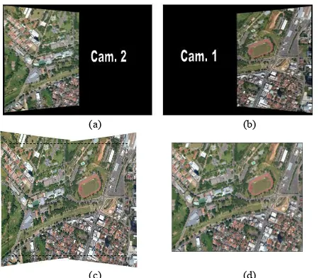
Firstly, the dimensions and the corners of the rectified image are defined, by using the inverse collinearity equations. Then, the pixel size is defined and the relations of the rectified image with the tilted image are computed with the collinearity equations. The RGB values of each pixel on the rectified image are interpolated in the projected position in the tilted image. The value used for the projection plane is the focal length of the camera 1 (Figure 1.a and 1.b).
(a) (b)
(c) (d)
Figure 1. Resulting rectified images of dual cameras: (a) left image from camera 2 and, (b) right image from camera 1 (c)
resulting fused image from two rectified images after registration and, (d) cropped without the borders.
(3) Image registration
(LSM). Ideally, the coordinates of these points should be the same, but owing to different camera locations and uncertainties in the EOP and IOP, discrepancies are unavoidable. The average values of discrepancies can be introduced as translations in row and columns to generate a virtual image. The standard deviations of these discrepancies can be used to assess the overall quality of the fusion process and standard deviations smaller than 1-2 pixels can be obtained without significant discrepancies in the seam-line.
When the standard deviations of the discrepancies in tie points coordinates are higher than a predefined threshold (e.g. 2 pixels) a scale factor can be computed from two corresponding tie points in the limits of the overlap area. This scale factor is used to compute a new projection plane distance and the right image is rectified again. The registration process is repeated to compute new discrepancies in the tie points coordinates and to check their standard deviations.
(4) Images fusion
The fourth step is the images fusion, when virtual images are generated (Figures 1.c and 1.d). The average discrepancies values in rows and columns of tie points are used to correct each pixel coordinates assigning RGB values for the pixels of the final image. Radiometric correction is also applied based on the differences in R, G and B values in tie point areas.
4. EXPERIMENTAL ASSESSMENT
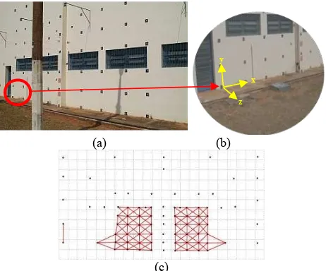
Two Fuji FinePix S3Pro RGB cameras, with a nominal focal length of 28 mm, were used in the experiments. Firstly, the system was calibrated in a terrestrial test field consisting of a wall with signalized targets (Figure 3.a). Several experiments were conducted to assess the results with distinct approaches and to check their effects in the rectified images and in the virtual fused images. The dual camera system in depicted in Figure 2 and camera technical data are given in Table 1.
(a) (b)
Figure 2.(a) Dual head system with two Fuji S3 Pro cameras (b) example of virtual images generated with the dual system.
Cameras Fuji S3 Pro
Sensor CCD – 23.0 x 15.5mm
Resolution 4256 x 2848 pels (12 MP)
Pixel size (mm) 0.0054
Focal length (mm) 28.4
Table 1. Technical details of the camera used.
Forty images, collected in five distinct camera stations, were used (16 for each camera). The image coordinates of circular targets were extracted with subpixel accuracy using an interactive tool that computes the centroid after automatic threshold estimation. Five exposure stations were used, and in
each station, eight images were captured (four for each camera), with the dual-mount rotated by 90º, -90º and 180º. After eliminating images with weak point distribution, 37 images were used: 18 images taken with camera 1 and 19 with camera 2; 8 images of camera 1 matched to corresponding images acquired with camera 2, with the result that 8 pairs were collected at the same instant, for which the RO constraints were applied.
In the experiments reported in previous papers (Tommaselli et al., 2009, 2010) calibration were performed with known object space coordinates, measured with topographic intersection methods. However, the accuracies of such a set of coordinates (σ ~ 3 mm) were not suitable to make feasible the analysis of the effects of RO constraints. In order to avoid this data, self calibrating bundle adjustment was used to compute parameters with a set of seven minimum absolute constraints. The 3D coordinates of one target, the X and Z coordinates of a second one and the Y and Z of a third one were introduced as absolute constraints. The X coordinate of the second point was measured with a precision calliper with an accuracy of 0.1mm.
A set of distances (131) between signalized targets (Figure 3.c) were measured with a precision calliper with an accuracy of 0.1mm, and these distances were used to check the results of the calibration process. After bundle adjustment the distances between two targets can be computed from the estimated 3D coordinates and compared to the distances directly measured.
(a) (b)
(c)
Figure 3. (a) Image of the calibration field; (b) origin of the arbitrary object reference system; and (c) existing targets and distances directly measured with a precision calliper for quality
control.
To assess the proposed methodology with real data, seven experiments were carried out, without and with different weights for the RO constraints. The experiments were carried out with RRMSC (Relative Rotation Matrix Stability Constraints - Equations 6 to 8) and BCSC (Base Component Stability Constraint - Equations 11), but varying the weights in the constraints. The two cameras were also calibrated in two separated runs (Experiment A) and in the same bundle system, but without RO constraints (Experiment B). In the experiments C to G, RO constraints were introduced with different weights, considering different variations admitted for the angular elements. Table 2 summarizes the characteristics of each experiment.
x y
Exp. A1 and A2 B C D E F G
Table 2. Characteristics of the seven experiments with real data.
Figure 4 presents the RMSE (Root Mean Squared Error) of the discrepancies in the 131 check distances for all the experiments. It can be seen that the errors in the check distances were slightly higher in the experiments with RO constraints. This result can be explained by the restriction imposed by the RO constraints, which enforce a solution that does not fit well for all the object space points.
Figure 4. RMSE of the check distances.
In Figure 5 the estimated standard deviations for some of the IOP (f, x0 and y0) for both cameras are presented for each experiment. It can be seen that the similar estimated standard deviations were achieved in all experiments, except when the cameras were calibrated independently.
Figure 5. Estimated standard deviations of f, x0 and y0 for both cameras.
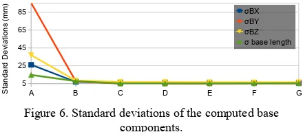
The base components were then computed from the estimated EOP (Equation 10) for those pair of images that received stability constraints (6 pairs). The average values and their standard deviations were computed to assess how these values were estimated. Figure 6 depicts the standard deviations of the base components for all experiments. It can be seen that precise values are achieved when introducing the base components stability constraints not affecting significantly the estimation of IOP and the overall accuracy of the bundle adjustment.
Figure 6. Standard deviations of the computed base components.
The relative rotation matrices for the same 6 image pairs for all experiments were also computed with Equation 3. The average values for the angles were then computed with their standard deviations, which are presented in Figure 7. It can be seen that
the standard deviation of the RO angles are compatible with the admitted variations, imposed with the Relative Rotation Matrix Stability Constraints (RRMSC). Experiments A and B, without constraints presented values with high standard deviations, as expected.
Figure 7. Standard deviations of rotation elements of the Relative Rotation matrix computed from estimated EOP.
The second part of the experiments were performed with aerial images taken with the same dual arrangement with flying height of 1520 m and a GSD (Ground Sample Distance) of 24 cm. The IOP and EOP computed for each experiment were then used to produce virtual images from the dual frames acquired in this flight. Five image pairs in a single strip were select with the aim of analysing the processes of registration and image fusion.
Firstly, image pairs were rectified using those IOP estimated in the self-calibration process with terrestrial data, for each group of experiments. Then, tie points were located in the overlap area of pairs of the rectified images using area based correspondence methods (minimum of 20 points for each pair). The average values of discrepancies and their standard deviations are then computed for each images pair. In Figure 8 the standard deviation of the discrepancies in the tie points coordinates (columns and rows) between the rectified image pairs are presented. These deviations show the quality of matching when mosaicking the dual images to generate a virtual image. It can been seen that fusion using parameters generated by self-calibration without constraints (experiments A and B) presents residuals with a standard deviation around 1.3 pixels in columns and 1 pixels in rows. The matching of the rectified image pairs when using parameters generated by self-calibration with RO constraints is better, mainly in experiments C and D (angular variations of 1” and 10”, respectively). The effects of varying the weight in the base components constraints were not assessed in these experiments.
Figure 8. Average values for the standard deviations of discrepancies in tie points coordinates of 5 rectified image pairs
with different sets of IOP and ROP.
Figure 9. Average values for the standard deviations of discrepancies in tie points coordinates of 5 rectified image pairs
with different sets of IOP and ROP, after scale change in the right image.
The distances between tie points in the overlap area were used to compute the scale factor and also to generated new rectified
images for the right camera. The process of measuring tie points and compute discrepancies and their standard deviations was repeated and the average values of the standard deviations are shown in Figure 8. The results were not significantly improved and the fusion is still better with parameters generated with ROP constraints.
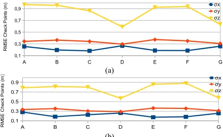
Virtual images generated for all experiments were then used in a bundle block adjustment and the results were assessed with independent check points. From the set of virtual images generated, three images were selected (Fig. 2.b), with six control points and 23 check points. These points were measured interactively with LPS (Leica Photogrammetric Suite) in a reference project. Then, the image points were transferred automatically with image correlation to all images of the experiments, ensuring that the same points were used. The RMSE in the check points coordinates are presented in Figure 10.a and 10.b. Fig. 10.a presents the results for the images generated without scale correction of the right image, whilst Fig. 10.b presents the values of the RMSE for the images generated with the right images corrected with a scale change.
(a)
(b)
Figure 10. RMSE in the check points coordinates obtained in a bundle adjustment with 3 virtual images generated with parameters obtained in the experiments: (a) without and (b) with scale correction in the right image.
The RMSE in check points coordinates were around 1 GSD (X and Y) and 2 GSD (Z) for the experiments D and G. The values for the RMSE in Z were higher in the other experiments (around 3 GSD for Z). In general, it can be concluded that the proposed process works successfully, achieving results similar to a conventional frame camera with a single sensor.
5. CONCLUSIONS
In this paper a set of techniques for dual head camera calibration and virtual images generation were presented and experimentally assessed. Experiments were performed with Fuji FinePix S3Pro RGB cameras. The experiments have shown that the images can be accurately rectified and registered with the proposed approach with residuals smaller than 1 pixel, and they can be used for photogrammetric projects. The calibration step was assessed with distinct strategies, without and with constraints considering the stability of Relative Orientation between cameras. In comparison with the approach presented in previous papers, some improvements were related to the constraints in the base components, instead on the base length constraint and also the use of self-calibration with distances check.
The advantage of the proposed approach is that an ordinary calibration field can be used and no specialized facilities are required. The same approach can be used in other applications,
like generation of panoramas, a suggestion that can be assessed in future work.
6. REFERENCES
Brown, D.C., 1971. Close-Range Camera Calibration,
Photogrammetric Engineering, 37(8), pp. 855-866.
Clarke, T.A., and J.G. Fryer, 1998. The development of camera calibration methods and models, Photogrammetric Record, 16(91), pp. 51-66.
Doerstel, C., W. Zeitler, and K. Jacobsen, 2002. Geometric calibration of the DMC: method and results. In: Proceedings of the ISPRS Commission I / Pecora 15 Conference, Denver, (34)1, pp. 324–333.
El-Sheimy, N., 1996. The Development of VISAT - A Mobile Survey System For GIS Applications, Ph.D dissertation, The University of Calgary, Calgary, Alberta, 175p.
Habib, A., M. Morgan, 2003. Automatic calibration of low-cost digital cameras, Optical Engineering, 42(4), pp. 948-955. He, G., K. Novak, and W. Feng, 1992. Stereo camera system calibration with relative orientation constraints. In: Proceedings of SPIE Videometrics, Boston, MA , Vol. 1820, pp. 2-8. King, B., 1994. Methods for the photogrammetric adjustment of bundles of constrained stereopairs. In: The International Archives of Photogrammetry and Remote Sensing, 30, pp. 473– 480.
King, B., 1995. Bundle adjustment of constrained stereopairs- mathematical models. Geomatics Research Australasia, 63, pp. 67-92.
Mostafa, M. M. R., and Schwarz, K. P., 2000. A Multi-Sensor System for Airborne Image Capture and Georeferencing.
Photogrammetric Engineering & Remote Sensing, 66(12), pp. 1417-1423.
Petrie, G., 2009. Systematic Oblique Aerial Photography Using Multiple Digital Frame Camera, Photogrammetric Engineering & Remote Sensing, 75(2), pp. 102-107.
Ruy, R. S., Tommaselli, A. M. G, Galo, M., Hasegawa, J. K., Reis, T. T. 2012. Accuracy analysis of modular aerial digital system SAAPI in projects of large areas. In: Proceedings of EuroCow2012 - International Calibration and Orientation Workshop. Castelldefels, Spain.
Tommaselli, A. M. G., Galo, M., Bazan, W. S., Marcato Junior, J. 2009. Simultaneous calibration of multiple camera heads with fixed base constraint In: Proceedings of the 6th International Symposium on Mobile Mapping Technology, 2009, Presidente Prudente, Brazil.
Tommaselli, A. M. G., Galo, M., Marcato Junior, J., Ruy, R. S., Lopes, R. F., 2010. Registration and Fusion of Multiple Images Acquired with Medium Format Cameras In: Canadian Geomatics Conference 2010 and the International Symposium of Photogrammetry and Remote Sensing Commission I, Calgary, Canada.
Zhuang, H., 1995. A self-calibration approach to extrinsic parameter estimation of stereo cameras. Robotics and Autonomous Systems, 15(3), pp. 189-197.
Acknowledgements
The authors would like to acknowledge the support of FAPESP (Fundação de Amparo à Pesquisa do Estado de São Paulo) with grant n. 07/58040-7. The authors are also thankful to CNPq for supporting the project with grants 472322/2004-4 and 305111/2010-8.
A B C D E F G
0,1 0,3 0,5 0,7
0,9 σxσy
σz
R
M
S
E
C
h
e
c
k
P
o
in
ts
(
m
)
A B C D E F G
0.1 0.3 0.5 0.7
0.9 σxσy
σz
R
M
S
E
C
h
e
c
k
P
o
in
ts
(
m