DEM GENERATION WITH WORLDVIEW-2 IMAGES
G. Büyüksalih a, I. Baz a, M. Alkan b, K. Jacobsen c
a
BIMTAS, Istanbul, Turkey - (gbuyuksalih, ibaz-imp)@yahoo.com b
Zonguldak Karaelmas University, Zonguldak, Turkey –[email protected] c
Institute of Photogrammetry and GeoInformation, Leibniz University Hannover, Germany – [email protected]
Commission I, WG I/4
KEY WORDS: Mapping, Space, Imagery, Matching, DEM/DTM
ABSTRACT:
For planning purposes 42km coast line of the Black Sea, starting at the Bosporus going in West direction, with a width of approximately 5km, was imaged by WorldView-2. Three stereo scenes have been oriented at first by 3D-affine transformation and later by bias corrected RPC solution. The result is nearly the same, but it is limited by identification of the control points in the images. Nevertheless after blunder elimination by data snooping root mean square discrepancies below 1 pixel have been reached. The root mean square discrepancy at control point height reached 0.5m up to 1.3m with a base to height relation between 1:1.26 and 1:1.80.
Digital Surface models (DSM) with 4m spacing have been generated by least squares matching with region growing, supported by image pyramids. A higher percentage of the mountainous area is covered by forest, requiring the approximation based on image pyramids. In the forest area the approximation just by region growing leads to larger gaps in the DSM. Caused by the good image quality of WorldView-2 the correlation coefficients reached by least squares matching are high and even in most forest areas a satisfying density of accepted points was reached.
Two stereo models have an overlapping area of 1.6 km times 6.7km allowing an accuracy evaluation. Small, but nevertheless significant differences in scene orientation have been eliminated by least squares shift of both overlapping height models to each other. The root mean square differences of both independent DSM are 1.06m or as a function of terrain inclination 0.74m + 0.55m tangent (slope). The terrain inclination in the average is 7° with 12% exceeding 17°. The frequency distribution of height discrepancies is not far away from normal distribution, but as usual, larger discrepancies are more often available as corresponding to normal distribution. This also can be seen by the normalized medium absolute deviation (NMAS) related to 68% probability leve l of 0.83m being significant smaller as the root mean square differences. Nevertheless the results indicate a standard deviation of the single height models of 0.75m or 0.52m + 0.39 tangent (slope), corresponding to approximately 0.6 pixels for the x-parallax in flat terrain, being very satisfying for the available land cover. An interpolation over 10m enlarged the root mean square differences of both height models nearly by 50%.
1. INTRODUCTION
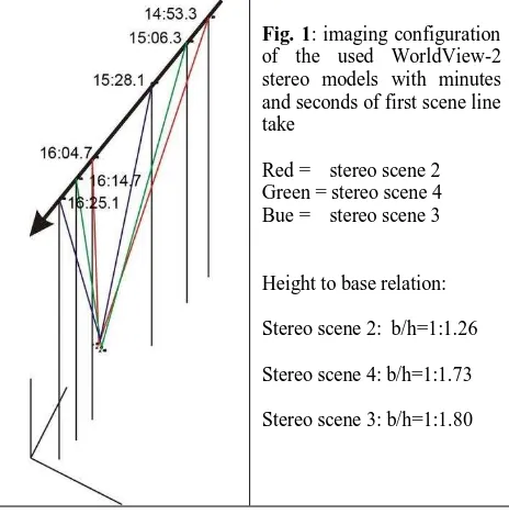
The very high resolution optical satellite WorldView-2 has the advantage of fast rotation, allowing an imaging of the three required stereo scenes from the same orbit (Fig. 1).
Fig. 1: imaging configuration of the used WorldView-2 stereo models with minutes and seconds of first scene line take
Red = stereo scene 2 Green = stereo scene 4 Bue = stereo scene 3
Height to base relation:
Stereo scene 2: b/h=1:1.26
Stereo scene 4: b/h=1:1.73
Stereo scene 3: b/h=1:1.80
Three pan-sharpened RGB image stereo pairs from June 6th, 2011, generated within 92 seconds; corresponding to an orbit distance of 687km or a footprint distance of 613km have been used. Only limited shadows can be seen caused by 68° sun elevation. The nadir angle of the scenes varies between 27° and 11°.
The images have been taken with 13 and 24 seconds time interval respectively with 10 and 11 seconds time interval. Only one image has been taken in the reverse scan direction. Between the last image of the forward view and the first of the backward view there is 37 seconds time interval (see figure 1).
Fig. 2: location of the three used WorldView-2 models
The images of the individual scenes are divided in up to 14 tiles which have been merged together based on the tile-file to simplify the image matching. A rough overlay of the left hand International Archives of the Photogrammetry, Remote Sensing and Spatial Information Sciences, Volume XXXIX-B1, 2012
images of the stereo models is shown in figure 2. The center and the right hand stereo models have a satisfying overlap allowing a comparison of the generated height models.
The image orientations are based on ground control points (GCPs) which have been used for the orientation of aerial images. The object coordinates of these GCPs are accurate, but the identification in the WorldView images with 50cm ground sampling distance (GSD) was very difficult, limiting the accuracy and causing some blunders.
2. SCENE ORIENTATION
Together with the scenes rational polynomial coefficients (RPC) are delivered describing the relation between the image and the ground coordinates based on the direct sensor orientation. The direct sensor orientation is not accurate enough for the required digital elevation models so the orientations have been determined by bias corrected RPC-solution using the GCPs for the correct location (Grodecki 2001, Jacobsen 2007).
RMSX RMSY Shift X Shift Y
2A 0.22 m 0.30 m -1.32 m 1.10 m
3A 0.49 m 0.60 m 2.84 m 3.23 m
4A 0.43 m 0.33 m 9.28 m 18.85 m
2B 0.44 m 0.63 m -1.17 m 0.72 m
3B 0.39 m 0.53 m -0.92 m -13.32 m
4B 0.27 m 0.13 m 2.24 m -13.74 m
Tab. 1: root mean square discrepancies at GCPs and shift determined by bias correction
The bias corrected RPC adjustment of the WorldView-2 scenes by the Hannover program RAPORI required a blunder correction by data snooping because of several misidentifications of the GCPs; finally between 9 and 16 GCPs have been used for the individual scene orientation resulting in average root mean square difference slightly better as the GSD (table 1). The bias correction required a 2D-affine transformation – just a shift was not satisfying and the individual affine coefficients have been in most cases significant.
An intersection of the models based on the individually determined scene orientation resulted in 0.60m root mean square discrepancies in the height (see also figure 3).
By bias correction a shift for the scene center is computed. This shift shows a not expected variation for the individual scenes from -1.32m up to 9.28m for X and -13.74m up to 18.85m for Y or in the root mean square 4.1m for X and 11.1m for Y (Tab. 1). Because of required upgrade of the used own program at first the orientation was handled by 3D affine transformation resulting in nearly the same result because of the sufficient number and distribution of the GCPs.
Fig. 3: discrepancies at GCPs in the three models
3. IMAGE MATCHING
The project area is partially urban with small cities and villages, includes a smaller percentage of agriculture areas, nearly 50% forest and several smaller lakes. The height ranges from sea level up to approximately 250m. The terrain is mountainous with an average slope of 12% (figure 4).
Fig. 4: distribution of terrain inclination
The image matching has been done with grey value images, generated from the RGB-images, by the Hannover program DPCOR which is based on least squares matching with region growing. As approximation seed points (corresponding points in both images of the stereo pair) are required. From the seed points the least squares matching grows to the neighbourhood up to totally filling the handled sub-area. This method works very well in open and build up areas with not too high buildings, but it had problems in the forest areas. By this reason in a first step the images have been scaled down linear by factor 10. With the scaled down images the region growing worked very well. The so determined corresponding image points have been used as seed points for the full resolution images. This corresponds to a pyramid method for the approximations with just two levels being different by linear scale factor 10. For the least squares matching only points having a correlation for the used window of 1010 pixels above a correlation threshold of 0.6 have been accepted.
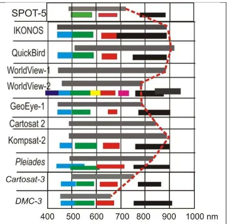
Fig. 5: spectral range of high resolution optical satellites International Archives of the Photogrammetry, Remote Sensing and Spatial Information Sciences, Volume XXXIX-B1, 2012
The spectral range of the high resolution panchromatic band of the latest very high resolution satellites WorldView-2 and GeoEye-1 has been reduced against IKONOS and QuickBird, but also WorldView-1 (figure 5). With the spectral range more close to the real panchromatic character, corresponding to the visible range, the pan-sharpening is simpler, but the image matching in forest areas becomes more difficult. Very high resolution images still have more problems in forest because of the strong height variation within the handled sub-matrixes, but even with lower resolution images without sensitivity in the near infrared range the automatic image matching in forest areas is difficult because of limited grey value range (Büyüksalih, Jacobsen 2005). The grey value variation in forest areas is not as poor as for SPOT-5; nevertheless the standard deviation of the grey values in forest areas in the used WorldView-2 images where the correlation coefficients are not reaching 0.6 usually is below +/-10 grey values.
Fig. 6: frequency distribution of correlation coefficient (area of figure 8), horizontal: correlation coefficient, vertical: frequency
As it can be seen at the example of figure 6, approximately 8% of the possible points are neglected in this sub-area if a threshold of 0.6 instead of 0.4 will be used for the correlation coefficient. Nevertheless by comparing figures 8 and 9 it is obvious that these points are dominantly located in forest areas.
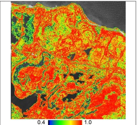
Fig. 7: color coded size of correlation coefficients in the overview image with 5m GSD, in grey = used image for matching in the area with correlation < 0.6
The correlation coefficients for matching one of the overview images, downscaled by linear factor 10, graphically presented in figure 7, are close to 1.0 in urban and village areas as in the range of the road network. It is smaller in agriculture areas and is often below 0.6 in forest areas. Of course the matching fails in water bodies. The areas with correlation coefficients below
0.6 in figure 7 are dominated by water bodies, on right hand side it is outside the stereo coverage, but the other parts are belonging to forest. In the not matched forest areas the standard deviation of the grey values is just in the range of 2 up to +/-10 grey values and this is a too low value for a correlation coefficient above 0.6.
Fig. 8: color coded size of correlation coefficients in a sub-area matched with 0.5m GSD images, correlation threshold =0.6, in grey = used image for matching in the not accepted area
Fig. 9: color coded size of correlation coefficients in a sub-area matched with 0.5m GSD images, correlation threshold =0.4, in grey = used image for matching in the not accepted area
With a threshold for the correlation coefficient of 0.4 (figure 9) instead of 0.6 (figure 8) the forest areas are quite better covered by accepted points. Nevertheless for the project the height of the bare ground was required and this is not possible by matching in closed forest areas. Even by filtering in forest areas the ground height cannot be achieved if no point is located on the ground. In addition in this mountainous area the tree heights are too different to allow a reduction of the tree crown height by a constant value to the ground. So there was no reason to reduce the correlation coefficient threshold to 0.4.
4. DEM ACCURACY ANALYSIS
Based on the corresponding image coordinates by intersection a digital elevation model (DEM) with a point spacing of approximately 4m was generated. The intersection was quite successful with root mean square parallaxes in the range of 0.2 up to 0.3m (0.4 – 0.6 pixels).
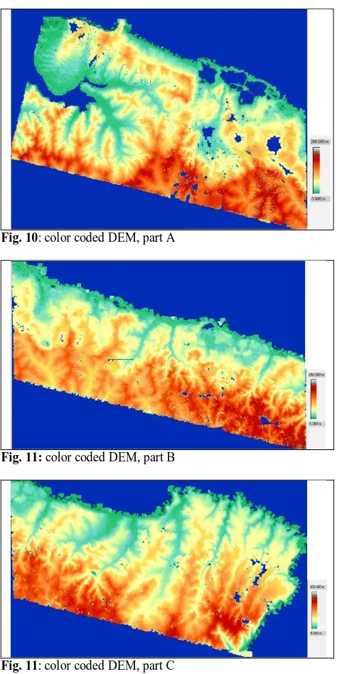
Fig. 10: color coded DEM, part A
Fig. 11: color coded DEM, part B
Fig. 11: color coded DEM, part C
20% of the DEM part B has an overlap with the DEM part C. This overlap is based on different images and different image orientations which is using different GCPs. So the three DEMs nearly independent determined. The conditions for comparing the overlapping DEMs are optimal, we have the same illumination and the viewing from the side (see figure 1) is also nearly the same. By matching digital surface models (DSMs) with the height of the visual surface are generated. But this is the same for the overlapping area, allowing the determination of the system accuracy which is disturbed in most cases, but not here by vegetation and buildings. The point location is not exactly the same, requiring an interpolation for the comparison
within the grid spacing of 4m. The overlapping DEMs are based on different GCPs having identification accuracy not better as 0.5m. This caused a small shift of one DEM against the other, determined by adjustment with the Hannover program DEMSHIFT. By DEM shifting the root mean square differences have been reduced by 10cm.
RMSZ: 1.06 BIAS: -.12
USED NUMBER OF DIFFERENCES: 411356 RMSZ WITHOUT BIAS : 1.05
RMSZ EUKLID: 1.04 WITHOUT BIAS 1.03 MEDIUM ABSOLUTE DEVIATION RELATED TO BIAS: .56 NMAD=MAD RELATED TO 68% PROBABILITY LEVEL: .83 Tab. 2: accuracy information of program DEMANAL
The comparison of the overlapping height models is based on 411356 points. The root mean square height difference is 1.06m with the same probability for deviations from both DEMs, so for a single DEM the accuracy can be estimated with 1.06/1.41= 0.75m. Corresponding to the average base to height relation of 1:1.5 a root mean square difference for the x-parallax of 0.5m or 1 pixel can be estimated. The small bias of 0.12m has just 1cm influence to the root mean square Z-difference. The Euklidian accuracy (shortest distance between both DEMs – perpendicular to the surface) is just 1cm below the root mean square z-difference. The discrepancies are not normal distributed as it can be seen by the normalized medium absolute deviation (NMAD) of 0.83m being clearly below the root mean square differences. As shown in figure 12, the frequency distribution of the height differences is slightly wider as a normal distribution and includes also some larger height differences, influencing the root mean square more as the NMAD.
Fig. 12: frequency distribution of height differences between overlapping stereo models
Fig. 13: root mean square height discrepancies depending upon terrain inclination
A reason for the slight misfit of the height discrepancy distribution to normal distribution can be seen in figure 13. The size of height discrepancies clearly depends upon the terrain inclination. The root mean square differences are smaller for flat terrain as for inclined terrain. The function shown in figure 13 can be described by: RMSZ = 0.74m + 0.55m tangent (slope). This adjusted function respects the number of discrepancies in the individual slope group, which is larger for not so much inclined terrain as for stronger inclined terrain (figure 4) – also demonstrated by the noise for stronger inclined areas exceeding tangent (slope) of 0.4. This linear dependency upon the terrain slope is typical for all height models.
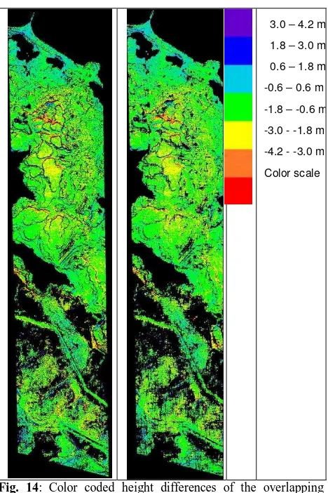
There is no tendency of the discrepancies upon the aspects (North-direction of inclination). The discrepancies are not larger or smaller for any North-direction of the terrain slope as it is height models – left original, right after filtering
The size of the height discrepancies between the overlapping height models is not equal distributed (figure 14); it is depending upon the terrain slope and the contrast in the different parts.
The height models include several small elements not belonging to the bare ground as single trees and small buildings, but especially in the forest area and surrounding the forest. These small elements are influencing the accuracy analysis by the required interpolation of the points not having exactly the same X,Y-location in both compared DEMs. By filtering with program RASCOR the number of small elements has been reduced (figure 14 right hand side and 15). This resulted in a reduction of the root mean square difference of both DEMs
from 1.06m to 0.92m or as function of the terrain inclination to RMSZ = 0.67m + 0.44mtan(slope).
Fig. 15: 3D shaded view to the overlapping DEM-part after filtering, three times exaggerated
CONCLUSION
The orientation of the six scenes was only slightly influenced by the problems of the control point identification. In general the caused by the threshold for the correlation coefficient of 0.6 and the reduced spectral sensitivity of the WorldView-2 panchromatic images to the near infrared range reducing the variation of the grey values in the forest areas. The intersection of the corresponding image points resulted in root mean square parallaxes of 0.4 up to 0.6 pixels.
The accuracy of the generated DEMs determined by comparing overlapping DEMs from neighbored stereo scenes is in the range of 0.75m for a single scene or even at 0.65m after filtering or for the flat parts at 0.52m respectively at 0.47m after Validation based on Optical Satellite Systems, EARSeL workshop 3D-remote sensing, Porto, 2005, http://www.ipi.uni-hannover.de/uploads/tx_tkpublikationen/DGVbuy.pdf (March 2012)
Grodecki, J., 2001: IKONOS Stereo Feature Extraction – RPC Approach, ASPRS annual conference St. Louis 2001
Jacobsen, K., 2007: Orientation of high resolution optical space images, ASPRS annual conference, Tampa 2007