LAND COVER INFORMATION EXTRACTION USING LIDAR DATA
Ahmed Shaker a, *, Nagwa El-Ashmawy aba Ryerson University, Civil Engineering Department, Toronto, Canada - (ahmed.shaker, nagwa.elashmawy)@ryerson.ca b
Survey Research Institute, National Water Research Center, Cairo, Egypt
Commission VII, WG VII/4 KEY WORDS: LiDAR, intensity data, Land Cover classification, PCA.
Light Detection and Ranging (LiDAR) systems are used intensively in terrain surface modelling based on the range data determined by the LiDAR sensors. LiDAR sensors record the distance between the sensor and the targets (range data) with a capability to record the strength of the backscatter energy reflected from the targets (intensity data). The LiDAR sensors use the near-infrared spectrum range which has high separability in the reflected energy from different targets. This characteristic is investigated to implement the LiDAR intensity data in land-cover classification. The goal of this paper is to investigate and evaluates the use of LiDAR data only (range and intensity data) to extract land cover information. Different bands generated from the LiDAR data (Normal Heights, Intensity Texture, Surfaces Slopes, and PCA) are combined with the original data to study the influence of including these layers on the classification accuracy. The Maximum likelihood classifier is used to conduct the classification process for the LiDAR Data as one of the best classification techniques from literature. A study area covering an urban district in Burnaby, British Colombia, Canada, is selected to test the different band combinations to extract four information classes: buildings, roads and parking areas, trees, and low vegetation (grass) areas. The results show that an overall accuracy of more than 70% can be achieved using the intensity data, and other auxiliary data generated from the range and intensity data. Bands of the Principle Component Analysis (PCA) are also created from the LiDAR original and auxiliary data. Similar overall accuracy of the results can be achieved using the four bands extracted from the Principal Component Analysis (PCA).
* Corresponding author:
Ahmed Shaker, Ryerson University, Department of Civil Engineering, 350 Victoria St., Toronto, Canada, M5B 2K3
E-mail: [email protected] Tel: +1 416 979 5000 (ext. 4658)
1. INTRODUCTION
Light Detection and Ranging (LiDAR) is a remote sensing technique used mainly for 3D data acquisition of the Earth surface and its applications in the 3D City modelling and building extraction and recognition, (Haala & Brenner, 1999, Song et al, 2002, Brennan and Webster, 2006, Hui et al., 2008, and Yan & Shaker, 2010). LiDAR sensors transmit laser pulses in near infrared (NIR) spectrum range toward objects and record the reflected energy. The distances between the LiDAR sensor and the targets (range data) are calculated. The 3D coordinates of the collected points are calculated from the range data with the aid of other sensors (GPS, and IMU), (Ackerman, 1999). LiDAR is considered as highly precise and accurate vertical and horizontal data acquisition system (Brennan and Webster, 2006). The high accurate data are used for generating digital elevation and/or surface models (DTM/DSM), Kraus & Pfeifer, (1998) used LiDAR data to create DTM in wooded areas. The accuracy of the DTM extracted was 25 cm for flat areas, which is improved to 10 cm by refining the data processing method.
In the last decade, substantial work is done to combine the LiDAR data with other external data such as aerial photos and satellite images for information extraction. Haala & Brenner (1999) combined LiDAR elevation data and a multi-spectral aerial photo (Green, Red and NIR bands) for building extraction using unsupervised classification technique. It was found that
combining the multi-spectral aerial photo with the LiDAR elevation data improved the classification results significantly.
LiDAR sensors not only record the time difference between sending and receiving signals; but they also record the backscattered energy from the targets (intensity data) in NIR spectrum range. A NIR image can be generated by interpolating the intensity data collected by the LiDAR sensors. With the capability to record the intensity of the reflected energy, definition of the classification of LiDAR data is not only referring to the separation of terrain and non-terrain features, but it includes the use of the intensity data for the classification of land covers as well. Hence, intensity data is investigated to be used to distinguish different target materials using various image classification techniques.
Recently, the use of the LiDAR intensity and range data has been studied for data classification and feature extraction. The intensity data were used primarily as a complementary data for data visualization and interpretation. LiDAR intensity data are advantageous over the multi-spectral remote sensing data in avoiding the shadows appear in the multi-spectral data. This is because LiDAR sensor is an active sensor. Hui et al., 2008, used the intensity and height LiDAR data for land-cover classification. Supervised classification technique was used to differentiate four classes: Tree, Building, Bare Earth and Low Vegetation. It was observed that combining the intensity data with the height data is an effective method for LiDAR data classification. However, quantitative accuracy assessment was not included in that research work.
Recent researchers combine the laser data with other auxiliary data such as multispectral aerial photos or satellite images, USGS DEM, texture data, normalized height, and multiple-returns data. Charaniya et al, (2004) used LiDAR height and intensity data, height variation data, multiple-return data, USGS DEM, and luminance data of a panchromatic aerial imagery for land-cover classification. A supervised classifier was used to distinguish four classes: trees, grass, roads, and roofs. The effect of band combinations on the classification results was studied. It was observed that height variation affected positively the classification results of the high vegetation areas, Luminance and intensity data was useful for distinguishing the roads from the low vegetation areas, and the multiple-return differences slightly improved the classification of roads and buildings but reduced the accuracy of the other classes.
Subsequently, researchers gave more attention to the intensity data and started to analyse the data and study different enhancing methods to remove the noise and improve the data interpretation. Song et al, (2002) examined different resampling techniques to convert LiDAR point data to grid image data which is filtered to remove the noise with minimum influence on the original data. The resampled grid is used to investigate the applicability of using the LiDAR intensity data for land-cover classification. It is concluded that the LiDAR intensity data contain noise that is needed to be removed.
Radiometric correction of the intensity data was suggested in some of the recent literatures (Coren and Sterzia, 2006; Höfle and Pfeifer, 2007). The process mainly relies on the use of the laser range equation to convert the intensity data into the spectral reflectance with consideration of the scanning geometry, the atmospheric attenuation, and the background backscattering effects. After the radiometric correction, the homogeneity of the land cover is improved and thus enhances the performance of feature extraction and surface classification. Yan et al. (2012) evaluated the accuracy of different land cover classification scenarios by using the airborne LiDAR intensity data before and after radiometric correction. An accuracy improvement of 8% to 12% was found after applying the radiometric correction.
This research investigates the use of the intensity data for land-cover information extraction. The Maximum Likelihood supervised classification technique is proposed and applied on two different study areas, and classification accuracy is assessed to recommend the most appropriate data combinations for such areas. The paper is divided into five sections. Section 1 is the introduction which highlights the previous work related to the use of LiDAR data in land cover information extraction. Section 2 comprises the methodology used in this research work. Section 3 describes the study areas and the datasets used. Section 4 includes the results of the experimental work and the analysis. The paper is concluded by a summary of the work and the future work in Section 5.
2. METHODOLOGY
The work is conducted in two main steps; data preparation, and data classification and assessment. In the data preparation step, the point data recorded by the LiDAR sensor are converted into raster image data, prepared as bands, to be used for the classification step. The bands prepared are also combined and Principal Component Analysis (PCA) is used to produce principal component bands for more investigation.
The second step is applying the classification algorithm on the different prepared datasets, and assessing the results. Four
information classes are identified in this study area. Details of the work procedure are discussed in the following sub-sections.
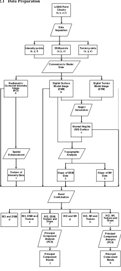
2.1 Data Preparation
Figure 1: Work Flow of Data Preparation
The data sets are prepared by converting the data collected by the sensor (range and intensity data) into raster image data. Since the multi-returned data are not available, the terrain has been separated manually from object surface by selecting the point data that falls on the roads and the terrain. The Kriging interpolation algorithm is used for point data conversion into image data. New image data (bands) are created representing
Heights (NH, calculated from the difference between the DSM and the DTM data). Other auxiliary image data (bands) are created to be used in the classification process. The auxiliary bands are: the texture from the intensity data, and the slope from both the DSM and the NH.
Several images are produced by combining two or more of the created bands. The image band combinations can be summarized as follows: bands of a) intensity and elevation, b) intensity, elevation and texture, c) intensity, elevation, texture, and slop.
The principal components are also created from the existing four bands to reduce the number of existing bands by eliminating the correlated ones. The classification analysis includes both datasets; the one created directly from the original LiDAR data (range and intensity), and the auxiliary datasets extracted from the original data. Figure 1 illustrates the work flow of the data preparation step.
2.2 Data Classification and Evaluation
The second part of the study work covers the classification process and the classification assessment of the results. The Maximum Likelihood classifier, as a supervised classification algorithm, is used with the bands created directly from the LiDAR data, and with the six band combinations mentioned above. The classification and evaluation is repeated for bands created from the PCA. The classification processes for all datasets (different band combinations) are summarized as follows:
1) Training signatures are identified for four different classes (trees, grass, buildings, and roads).
2) Statistical assessments of the training signatures are done and further enhancement to the selection of the training areas are taken place, if required.
3) Maximum Likelihood algorithm is applied and the image data is classified into the corresponding classes.
4) Assessment the results of the classification using ground truth data and by performing evaluation using error matrix. The classification process is evaluated using about 1000 reference points, for each study area, that are randomly selected from the original point cloud data to avoid the effect of the interpolation on the accuracy of the ground truth. The well-distributed points over the study area are randomly generated. The ground truth information is collected from the ortho-rectefied aerial photo provided with the LiDAR data. Finally, the accuracies achieved from classification results of the different band combinations are compared.
3. STUDY AREA AND DATA SETS 3.1 Study Area
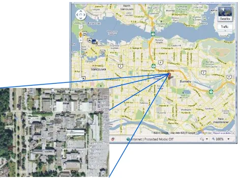
A study area is chosen, which covers a part of the British Columbia Institute of Technology (BCIT) located in the Burnaby, British Columbia, Canada (122°59’W, 49°15’N). An area of 500 m x 400 m is selected for the experimental work because it contains a variety of the land cover features on the ground including; buildings, parking areas, trees and open spaces with grassy coverage, (Figure 2 ).
Figure 2: Study Area (British Colombia Institute of Technology, Vancouver)
3.2 Data Sets
A Leica ALS50 sensor operating in 1.064 μm wavelength and 0.33 mrad beam divergence is used for the LiDAR acquisition mission on July 17, 2009 at local time 14:55. The flying height for this mission was around 600m. The data acquired contains a 3D point cloud (x, y, and z coordinates) and linearized intensity values (I) for each point.
a b
c d
Figure 3: a) Geometrically Calibrated and Radiometrically corrected Intensity Image, b) DSM, c) NH, and d) Ortho-rectified
Aerial Photo
The provided dataset for this experimental work is: an Ortho-rectified aerial photo for the study area, and geometrically calibrated and radiometrically corrected LiDAR data (including x, y, z and I), the aerial photo is acquired at the same time of the LiDAR data acquisition mission. The related geometrical calibration and radiometrical correction works are illustrated in Yan et. al. (2012). The LiDAR data (intensity and rang) are converted to raster image with pixel size equals to 20 cm to produce the intensity image and the DSM. The LiDAR points fell on the ground are separated, and a DTM is produced using these points with the same pixel size of 20 cm. The difference International Archives of the Photogrammetry, Remote Sensing and Spatial Information Sciences, Volume XXXIX-B7, 2012
between the DSM and the DTM is calculated to produce a normal heights raster image. Figure 3 a, b, and c illustrates the produced LiDAR raster image data (intensity, DSM, and Normal Height (NH), respectively). Figure 3d represents the ortho-rectified aerial photos for the study area.
4. RESULTS AND DISCUSSION
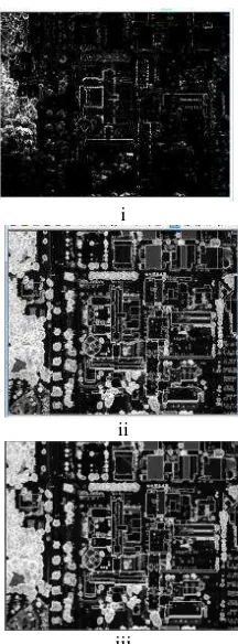
A close look to the data provided and the characteristics of the study area shows that the intensity values of the areas covered by vegetation (either trees or grass) are higher than those covered by man-made features (buildings and roads). This is expected from the reflectance characteristics of vegetation in Near Infra-Red range. It is also observed that the intensity of the areas covered by buildings and roads are more homogeneous than the intensity of trees and grass areas. Moreover, the tree areas have a larger variation in elevations compared to the buildings and road areas. Based on the previous observations, it is noted that intensity data can be effectively used for distinguishing man-mad features from vegetation fields. The texture of the intensity can be used for representing the homogeneity of the land covers, Figure 4 i. The slope of the elevation data can be used to represent the plane surfaces, such as buildings and roads, Figure 4 ii, and iii, for the DSM and NH respectively.
i
ii
iii
Figure 4: Bands created from range and intensity data i) Intensity Texture, ii) DSM slop, and iii) NH slope
The prepared raster LiDAR data are used individually for the land cover classification process, Figure 5. The image data bands used individually are: a) Intensity, b) DSM, and c) Normal Height. Additionally, six combinations of image bands are developed to examine the use of the auxiliary data on the classification results. The auxiliary band combinations are: d) Intensity and DSM, e) Intensity and Normal Heights (NH), f) Intensity, DSM, and Intensity Texture, g) Intensity, NH, and Intensity Texture, h) Intensity, DSM, Intensity Texture, and
DSM Slope, and i) Intensity, NH, Intensity Texture, and NH Slope. The results of land cover classification of all cases are shown in Figures 5, (cases a to i).
Trees
Buildings
Grass/ Bare Soil
Roads
(a)
(b) (c)
(d) (e)
(f) (g)
(h) (i)
(j) (k)
Figure 5: Results of Land Cover Classification
The principal components from the 4-bands (Intensity, DSM, Intensity Texture, and DSM Slope) are generated and classified (case j). Other principle components from the Intensity, NH, Intensity Texture, and NH Slope are also generated in order to test the effect of using the normal height instead of the DSM on International Archives of the Photogrammetry, Remote Sensing and Spatial Information Sciences, Volume XXXIX-B7, 2012
the land cover classification accuracy. The results of land cover classification of the PCA cases are shown in Figures 5, cases j and k.
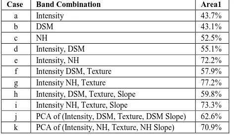
The overall accuracy calculated based on the 1000 ground truth points for all the cases is listed in Table 1. The results obtained show that the overall accuracy by using the intensity and the DSM data individually are less than 45%, (Table 1, case a, and b). Combining both the intensity and the DSM data improves the results to 55% (Table 1, case d). Using the normal height band individually does not improve the accuracy. This is because of the similarity between the heights of the trees and the buildings, as well as due to the similarity in heights between the roads and the grass. Nevertheless, combining the normal heights data with the intensity data has a significant improvement in the overall accuracy of the classification results.
An overall accuracy of about 70% can be achieved as it is seen in Table 1 (case e). It is also observed that the overall accuracy of the classification results is increased by combining the texture of the intensity data to the intensity and elevation data, (cases f and g using intensity texture comparing to cases d and e without using texture, respectively). Yet, combining the slope of the elevation data with the intensity, the elevation, and the texture data does not improve the overall classification accuracy. For the principle component analysis the accuracy of results comparable to the classification results combined images. Further work are planned to investigate more bands created from the LiDAR data.
Table 1: Accuracy assessments of the land cover classification
Case Band Combination Area1
a Intensity 43.7%
i Intensity NH, Texture, Slope 73.3%
j PCA of (Intensity, DSM, Texture, DSM Slope) 62.6%
k PCA of (Intensity, NH, Texture, NH Slope) 70.9%
5. CONCLUSIONS
This research work examines the use of the LiDAR data only (range and intensity data) for Land-Cover information extraction. Different image bands (Intensity, DSM, Normal Height, Intensity Texture, DSM Slope, and Normal Height Slope) are created from the LiDAR points recorded by Leica ALS50 sensor. In addition, components of the principle component analysis are generated to be used for the land cover classification process. LiDAR dataset covering an area of the British Columbia Institute of Technology (BCIT) is classified using the Maximum likelihood classifier, and around 1000 ground truth points were used for the accuracy assessment.
From the results obtained, it is observed that using the LiDAR original data (range and intensity) individually in the classification process introduce an overall accuracy of less than 45%. However, using both the range and the intensity data improves the results accuracy by approximately 10%. Adding auxiliary data, such as Texture of the intensity data and surfaces slope, slightly improves the accuracy of the land cover
classification. Using the normal heights as elevation data instead of the DSM, improves the accuracy of the classification results significantly, (from 55% to more than 72%).
Components of the Principle Component Analysis (PCA) created from the LiDAR original and auxiliary data can also be used. Similar overall accuracy to the results achieved by using the original and the auxiliary data can be achieved (about 70%). Further research work is underway to further investigate the PCA using more bands extracted from the LiDAR and other sensor data to improve the classification accuracy.
ACKNOWLEDGMENT
This research work is supported by the Discovery Grant from the Natural Sciences and Engineering Research Council of Canada (NSERC) and the GEOIDE Canadian Network of Excellence, Strategic Investment Initiative (SII) project SII P-IV # 72. The authors would like to thank McElhanney Consulting Services Ltd, BC, Canada for providing the real LiDAR and image datasets to the GEOIDE project.
6. REFERENCES
1. Ackerman, F., 1999. Airborne Laser Scanning-Present Status and Future Expectations. ISPRS Journal of Photogrammetry & Remote Sensing, 54, No. 2-3, pp. 64– 67.
2. Brennan, R., and Webster, T.L., 2006. Object-Oriented Land Cover Classification of LiDAR-derived Surfaces. Can. J. Remote Sensing, Vol. 32, No. 2, pp. 162–172. 3. Charaniya, A., Manduchi, R., and Lodha, S., 2004.
Supervised Parametric Classification of Aerial LiDAR Data. In: Proceedings of the 2004 IEEE Computer Society Conference on Computer Vision and Pattern Recognition Workshops (CVPRW’04).
4. Coren, F., and Sterzai, P., 2005. Radiometric Correction in Laser Scanning. International Journal of Remote Sensing, 27(15), pp. 3097 -3014.
5. Haala, N., Brenner, C., 1999. Extraction of Buildings and Trees in Urban Environments. ISPRS Journal of Photogrammetry & Remote Sensing, 54 (1999) 130–137. 6. Höfle, B., and Pfeifer, N., 2007. Correction of laser
scanning intensity data: Data and model-driven approaches. ISPRS Journal of Photogrammetry & Remote Sensing, 62(6): 415-433.
7. Hui, L., Di, L., Xianfeng, H., and Deren, L., 2008. Laser Intensity Used In Classification of LiDAR Point Cloud Data. Geoscience and Remote Sensing Symposium, Boston, Massachusetts, U.S.A.
8. Jensen, J., 2005. Introductory Digital Image Processing, 3/e, Prentice Hall, Upper Saddle River, New Jersey, ISBN 0-13-1453361-0: 526p.
9. Jollife, I.T., 1986. Principal Component Analysis. New York: Springer-Verlag.
10. Kraus, K., and Pfeifer, N., 1998. Determination of Terrain Models in Wooded Areas with Airborne Laser Scanner Data. ISPRS Journal of Photogrammetry & Remote Sensing, 53 (1998) 193–203.
11. Song, J., Han, S., Yu, K., and Kim, Y., 2002. Assessing the Possibility of Land-Cover Classification Using LiDAR Intensity Data. ISPRS Commission III, Symposium, Graz, Austria. P.B-259ff.
12. Yan, W., and Shaker, A., 2010. Radiometric Calibration of Airborne LiDAR Intensity Data for Land Cover International Archives of the Photogrammetry, Remote Sensing and Spatial Information Sciences, Volume XXXIX-B7, 2012
Classification. Canadian Geomatics Conference and Symposium of Commission I, ISPRS. Calgary, Alberta, Canada.
13. Yan, W.Y., Shaker, A., Habib, A., and Kersting, A. P. 2012. Improving Classification Accuracy of Airborne LiDAR Intensity Data by Geometric Calibration and Radiometric Correction. ISPRS Journal of Photogrammetry and Remote Sensing, 67(1), pp. 35-44