STATISTICAL METHOD TO OVERCOME OVERFITTING ISSUE IN RATIONAL
FUNCTION MODELS
S. H. Alizadeh Moghaddam a, *, M. Mokhtarzade a, A. Alizadeh Naeini b, S. A. Alizadeh Moghaddam a
a Faculty of Geodesy and Geomatics Engineering, Khaje Nasir Toosi University of Technology, Tehran, Iran-
[email protected], [email protected], [email protected]
b Dept. Geomatics, Faculty of Civil Engineering and Transportation, University of Isfahan, Isfahan, Iran - [email protected]
KEY WORDS: Rational Function Models (RFMs), Overfitting, Statistical test, Regularization
ABSTRACT:
Rational function models (RFMs) are known as one of the most appealing models which are extensively applied in geometric correction of satellite images and map production. Overfitting is a common issue, in the case of terrain dependent RFMs, that degrades the accuracy of RFMs-derived geospatial products. This issue, resulting from the high number of RFMs’ parameters, leads to ill-posedness of the RFMs. To tackle this problem, in this study, a fast and robust statistical approach is proposed and compared to Tikhonov regularization (TR) method, as a frequently-used solution to RFMs’ overfitting. In the proposed method, a statistical test, namely, significance test is applied to search for the RFMs’ parameters that are resistant against overfitting issue. The performance of the proposed method was evaluated for two real data sets of Cartosat-1 satellite images. The obtained results demonstrate the efficiency of the proposed method in term of the achievable level of accuracy. This technique, indeed, shows an improvement of 50–80% over the TR.
1. INTRODUCTION
Since 1999, High-Resolution Satellite Images have paved the way for extracting detailed and accurate information from our planet and nowadays, with no contest, remotely-sensed images are the main source of information. To this end, it is vital to know the mathematical relationship between the image and the object spaces (Tao & Hu, 2001). Sensor models, that can be grouped into physical and generic ones, define this relationship (Toutin, 2004).
Physical or rigorous sensor models, by which high geometric accuracy can be obtained, fully consider the procedure of the geometric imaging (Tao & Hu, 2001; Zhang et al., 2011); therefore, each of the model’s parameter has a physical meaning. Although physical models have the aforementioned benefits, they have their own drawbacks, including model complexity and sensor dependency, that is, each sensor has its own unique model (Long et al., 2015).
Of the various generic models, none has received more attention than Rational Function Models (RFMs) (Fraser et al., 2006). Habib et al. (2007) have revealed that RFMs is an appropriate alternative for the physical sensor model. The Open GIS Consortium (OGC), in addition, recommends this model (Long et al., 2015).
In order to use the RFMs, RFMs’ coefficients, called rational polynomial coefficients (RPCs) must be determined. Tao and Hu (2003) have proposed two methods, namely Direct and Iterative Least-Square (LS) solution, for RPCs estimation. Strictly speaking, to provide initial values for the Iterative LS solution, one may apply the Direct LS (DLS) method.
Among RFMs’ drawbacks overfitting is the most important one that degrades the both accuracy and efficacy of the RFMs. The over-fitting issue results from both the large number of RFMs’
* Corresponding author
parameters, and the strong correlation among them (Long et al., 2015; Naeini et al., 2017).
“Variable selection” (Draper et al., 1966) and “Regularization” (Poggio et al., 1985) are of methods applied to tackle the RFMs’ overfitting. Tikhonov regularization (TR), based on the L2-norm regularization, is the most common way to prevent overfitting and makes the RFMs’ normal matrix well-posed (Poggio et al., 1985).
In addition to the Variable selection and Regularization techniques , methods based on artificial intelligence such as Genetic Algorithm (GA) have been successfully applied to address the overfitting problem (Zoej et al., 2007). These methods, which are conceptually similar to Variable Selection, determine the optimum set of parameters which minimize the RMSE over Dependent Control Points (DCPs). These techniques, however, are very exhaustive from the computational point of view. In addition, their performance is highly dependent to some parameters which are usually set in a tedious trial-and error manner. More importantly, these methods cannot be robust because different results are obtained from different runs (Kurban et al., 2014).
The foregoing literature review indicates that the overfitting of the RFMs have attracted many attentions. However, the capability of the statistical tests, such as t-test, has not been considered in remote sensing and photogrammetry literature.
In this paper, a novel and robust method based on a statistical test is proposed to prevent overfitting issue. Our method, that has a simple concept and low computational burden, uses t-test in a recursive mode to remove those coefficients which are statistically insignificance.
The International Archives of the Photogrammetry, Remote Sensing and Spatial Information Sciences, Volume XLII-4/W4, 2017 Tehran's Joint ISPRS Conferences of GI Research, SMPR and EOEC 2017, 7–10 October 2017, Tehran, Iran
This contribution has been peer-reviewed.
The rest of the paper is organized in the following fashion. Theoretical background of the RFMs and its solutions are first reviewed. The exposition of the proposed method will be provided in the third section. In section 4, the experimental results together with a comprehensive discussion are given. Last section will be concluded some remarks.
2. THEORETICAL BACKGROUND
RFMs are of mathematical tools projecting a 2D image space into a 3D ground space. They model the spatial relationship between a pixel in the image, with two dimensional coordinates, and its corresponding point on the ground space. RFMs are actually a ratio between two polynomials. The variables of these functions are the ground space coordinates of a pixel (Fraser et al., 2006).
= , , / , , (1)
= , , / , , (2)
where (, ) are the normalized line and sample of a point in image space; ( , , ) are latitude, longitude, and height of the point in the ground space respectfully (Franklin, 2001).
{ λ and h are the geographic latitude, longitude, and height in the ground space; � , λ , and h are the offset values and ��, λ�, and h� are the corresponding scale factors.
Tao and Hu (2003) have proposed two methods, based on LS, to solve the RFMs. According to LS estimation method, unknown vector ̂ that contains RPCs will be approximated as follows:
̂ = � − � � (4)
= � [1 , 1 , … , 1 ,�1 ,�1 , … ,�1] (5)
Where the diagonal matrix can be seen as the weight matrix, is the design matrix, � is the observation vector, and � are the denominator values of Eqs. 1 and 2. More details are available in (Tao & Hu, 2001; Zhang et al., 2011).
Owing to the dependency of on ̂, unknown vector should be estimated in an iterative fashion. This method is named as “Iterative LS” RFMs solution in the literature (Tao & Hu, 2001). For the first iteration, is typically set as the identity matrix. The first iteration’s result is the “Direct LS (DLS)” solution for RFMs.
Making the normal matrix � well-posed, we can apply Tikhonov method as bellow:
̂ = � + �� − � � (6)
In which, � and � are the identity matrix and regularization parameter, respectively. � can be valued manually or via L-curve method (Hansen, 1992).
3. PROPOSED METHOD
To the best of our knowledge, capability of statistical tests for the prevention of the overfitting issue, particularly in the context of the RFMs has not been addressed in the literature. Models that include insignificance, i.e. extra/unnecessary parameters, are too flexible which results in an unstable oscillation. This issue is named overfitting. Since the estimated values of the insignificance parameters are typically closed to zero, statistical tests can be easily applied to examine if any unnecessary parameters have been included in the model.
To do so, a two-sided statistical test can be designed with the null hypothesis if each parameter is equal to zero. In the statistics scope, this test is named “significance test”. The test statistic ( �), which has a student’s t-distribution, is as follows:
�= �̂ � − (7)
�̂ =�� � (8)
�=�̂�̂�
� (9)
Where is the design matrix, is the observation weight, � is the covariance matrix of estimated parameters, � is the residual vector, represents the degree of freedom, and �̂ is called variance factor. �̂� is the estimated value of the i-th model’s parameter and � is its corresponding test statistic value. The diagonal elements of the matrix � are variances of the estimated parameters. Therefore, to calculate the standard deviation of the i-th estimated parameter (�̂� , square root of the i-th diagonal element must be calculated.
To sum up, for every estimated parameter, if the absolute value of its test statistic (| �|) is larger than the crucial value, extracted from t-distribution table with 1 −� as the upper cut-off value ( ��, −�
2), then the parameter is not statistically equal to zero (see Eq. 10) and, as a result, doesn't cause overfitting. The parameters which are not statically equal to zero can be preserved in the model.
| �| > ��, −� (10)
� is the cut-off value for the designed statistical test , in which �
is the significance level. Due to the symmetry of the t-distribution, only upper cut-off value will be considered (Brown & Melamed, 1990).
The International Archives of the Photogrammetry, Remote Sensing and Spatial Information Sciences, Volume XLII-4/W4, 2017 Tehran's Joint ISPRS Conferences of GI Research, SMPR and EOEC 2017, 7–10 October 2017, Tehran, Iran
This contribution has been peer-reviewed.
Figure 1. Flow chart of the proposed method
Figure 1 illustrates the flow chart of our method. Firstly, third-order RFM will be solved via Direct solution. Then, all of the seventy-eight estimated RPCs as well as their corresponding standard deviations are employed to examine if any parameters are statistically zero (Eqs. 7–10). Secondly, the statically zero parameters are omitted from the model. By doing this, a new RFM is made whose parameters need to be estimated. Parameters of the new model and their corresponding standard deviations are again used to identify and exclude statistically zero parameters. This procedure will be repeated until no statically zero parameter exists in the model.
4. RESULT AND DISCUSSION
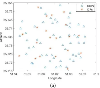
To validate the capability of the proposed method, two High-Resolution satellite images of Cartosat-1 sensor, with the ground sample distance of 2.5 meters, were applied. All of the GCPs, shown in Figure 2, were meticulously extracted from 1:2000 maps. The first and the second images were respectively acquired over Kermanshah, Iran and Tehran, Iran.
(a)
1 - Iterative Least-Square solution regularized via Tikhonov method
(b)
Figure 2. Distribution of GCPs and ICPs: (a) First data-set over Tehran, Iran; (b) Second data-set over Kermanshah, Iran.
The proposed method was compared to the Iterative LS solution, regularized with TR method (ILST). According to table 1, the ILST method is not substantially robust because its RMSE values of ICPs are greater than one pixel, especially in the second dataset. Note that the model, approximated via ILST method, was a third-order RFM that is frequently employed by the satellite imagery vendors.
Data set
GCPs /ICPs
Total ICPs’ RMSE (pix)
Total GCPs’ RMSE (pix) Proposed
method ILST1
Proposed
method ILST
1 55/21 0.84 1.72 6e-4 3e-4
2 60/20 0.87 4.21 8e-4 2e-4
Table 1. RMSE of the ICPs and GCPs
Moreover, Table 1 verifies the presence of the overfitting issue which is not been addressed completely by ILST method. As mentioned, the high number of RFMs’ parameters result in high flexibility of the RFMs, that means, the RFMs perfectly fit to GCPs, used for RFMs training. However, due to overfitting issue, it doesn't fit to new samples, including ICPs. The fourth and sixth columns of the Table 1 provide solid evidence for the pernicious effect of this issue.
The worst drawback of any Regularization method, including TR method, is the regularization parameter that must be set optimally. For this purpose, we applied the L-curve (Hansen, 1992), as a convolutional method (Ma et al., 2017).
GCPs
RFMs Direct solution
All terms are
non-zero?
Omit zero terms Approximate
new model
Non over fitted model
NO Yes
The International Archives of the Photogrammetry, Remote Sensing and Spatial Information Sciences, Volume XLII-4/W4, 2017 Tehran's Joint ISPRS Conferences of GI Research, SMPR and EOEC 2017, 7–10 October 2017, Tehran, Iran
This contribution has been peer-reviewed.
Figure 2. ICPs’ RMSE of both data sets
According to the RMSE values in both Table 1 and Figure 2, the proposed method outperforms ILST. For the first and second dataset, our method was respectively 50% and 80% more accurate than ILST. RMSE values of the proposed method, also, reached to the subpixel value for both datasets that is substantially satisfactory.
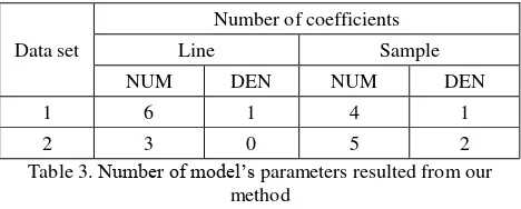
The subpixel value is caused by two reasons that demonstrate the efficacy of our method. Firstly, the designed RFM, based on the proposed method, is not influenced by the overfitting issue, due to the small number of parameters (see Table 3). Secondly, degree-of-freedom (df) of the designed model is much more than that of third-order RFM. Needless to mention that the large df
value leads to the reliable result.
Data set
Table 3. Number of model’s parameters resulted from our method
In addition to the aforementioned advantages, our method unlike TR method does not have any essential parameter to be set. The only parameter of the proposed method is the significance level � which can be easily set. In our experiments, we set it as � = 0.05 which is common when using any statistical tests.
5. CONCLUSION
Extracting essential products such as Digital Elevation Model (DEM) from satellite images, no one can deny the role of mathematical models that describe the relationship between the image and the ground spaces. For this purpose, RFMs have widely been applied. However, these models severely affected by the overfitting issue.
In this paper, we directly addressed the overfitting of the RFMs by means of a statistical test. The results prove the efficacy of our proposed method. Dealing with the aforementioned issue, our method was 50% to 80% more effective than the common Regularization method—TR method. In addition to the efficacy, compared to the Regularization based methods, our method needs no essential parameter to be optimally set.
Therefore, due to the capabilities of our method, it can be considered as an algorithm to cope with overfitting, and as a result, ill-posedness of the RFMs.
REFERENCES
Brown, S. R., & Melamed, L. E. (1990). Experimental design and
analysis: Sage.
Draper, N. R., Smith, H., & Pownell, E. (1966). Applied
regression analysis (Vol. 3): Wiley New York.
Franklin, S. E. (2001). Remote sensing for sustainable forest
management: CRC Press.
Fraser, C. S., Dial, G., & Grodecki, J. (2006). Sensor orientation via RPCs. ISPRS journal of Photogrammetry and Remote
Sensing, 60(3), 182-194.
Hansen, P. C. (1992). Analysis of discrete ill-posed problems by means of the L-curve. SIAM review, 34(4), 561-580.
Kurban, T., Civicioglu, P., Kurban, R., & Besdok, E. (2014). Comparison of evolutionary and swarm based computational techniques for multilevel color image thresholding. Applied Soft
Computing, 23, 128-143.
Long, T., Jiao, W., & He, G. (2015). RPC Estimation via L1-Norm-Regularized Least Squares (L1LS). IEEE Transactions on
Geoscience and Remote Sensing, 53(8), 4554-4567.
Ma, D., Tan, W., Zhang, Z., & Hu, J. (2017). Parameter identification for continuous point emission source based on Tikhonov regularization method coupled with particle swarm optimization algorithm. Journal of Hazardous Materials, 325, 239-250.
Naeini, A. A., Moghaddam, S. H. A., Mirzadeh, S. M. J., Homayouni, S., & Fatemi, S. B. (2017). Multiobjective Genetic Optimization of Terrain-Independent RFMs for VHSR Satellite Images. IEEE Geoscience and Remote Sensing Letters, 14(8), 1368-1372. doi:10.1109/LGRS.2017.2712810
Poggio, T., Torre, V., & Koch, C. (1985). Computational vision and regularization theory. nature, 317(6035), 314-319.
Tao, C. V., & Hu, Y. (2001). A comprehensive study of the rational function model for photogrammetric processing.
Photogrammetric engineering and remote sensing, 67(12),
1347-1358.
Toutin, T. (2004). Review article: Geometric processing of remote sensing images: models, algorithms and methods.
International journal of remote sensing, 25(10), 1893-1924.
Zhang, L., He, X., Balz, T., Wei, X., & Liao, M. (2011). Rational function modeling for spaceborne SAR datasets. ISPRS journal
of Photogrammetry and Remote Sensing, 66(1), 133-145.
Zoej, M. V., Mokhtarzade, M., Mansourian, A., Ebadi, H., & Sadeghian, S. (2007). Rational function optimization using genetic algorithms. International Journal of Applied Earth
Observation and Geoinformation, 9(4), 403-413.
0.84 0.87
The International Archives of the Photogrammetry, Remote Sensing and Spatial Information Sciences, Volume XLII-4/W4, 2017 Tehran's Joint ISPRS Conferences of GI Research, SMPR and EOEC 2017, 7–10 October 2017, Tehran, Iran
This contribution has been peer-reviewed.